Quantization in LLM Inference: Techniques, Tradeoffs, and What's Next

TL;DR

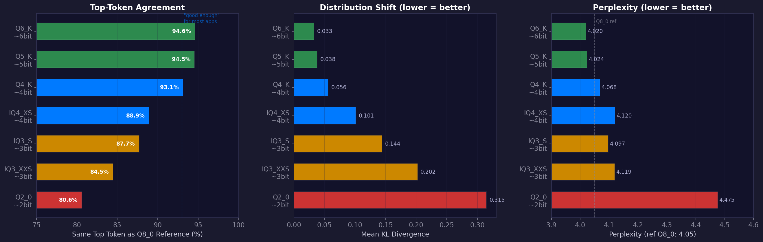
A 70-billion-parameter model in FP16 takes 140 GB of memory. A single H100 has 80 GB. Your laptop has 16. Quantization is the most important practical technique for closing that gap — not as a compromise, but as an engineered tradeoff where you give up precision you don’t need in exchange for memory and speed you desperately do. At 4-bit, a 70B model agrees with its 8-bit reference on the most-likely token 93% of the time — for most applications, indistinguishable. This post walks through how quantization works in real inference systems, why it works better than you’d expect, and where the field is heading — from data centers to robots.

---

What Quantization Actually Is

At its core, quantization replaces high-precision floating-point numbers with lower-precision representations.

A standard FP16 value uses 16 bits to represent a number. An INT8 value uses 8 bits. An INT4 value uses 4. The fewer bits, the less memory a model consumes, and the faster arithmetic can be — because memory bandwidth, not compute, is the bottleneck in LLM inference.

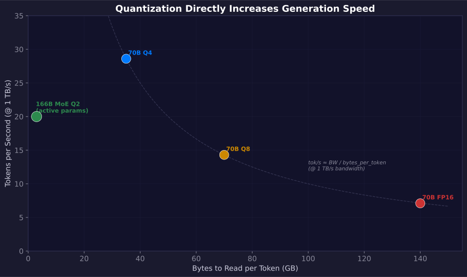
Consider the arithmetic: a 70B model generating one token needs to read all 70B parameters from memory once. At FP16 that’s 140 GB of data. An NVIDIA H100 has ~3.35 TB/s of memory bandwidth, so even at peak utilization, reading 140 GB takes ~42ms — that’s only ~24 tokens per second, and we haven’t done any math yet. At INT4, the same read is 35 GB, taking ~10ms. Quantization doesn’t just save space — it directly increases generation speed.

---

Step by Step: How Block Quantization Works

The simplest and most widely used form is symmetric block quantization. Let’s walk through it concretely.

Quantizing a block of 32 FP32 values to INT8

Input:  [0.23, -1.07, 0.84, 0.01, -0.56, ..., -0.41]   ← 32 floats = 128 bytes

Step 1: Find the absolute maximum
        amax = max(|values|) = 1.07

Step 2: Compute the scale factor
        scale = amax / 127 = 0.008425...

Step 3: Quantize each value
        q[0] = round(0.23  / 0.008425) = round(27.30)  = 27
        q[1] = round(-1.07 / 0.008425) = round(-127.0) = -127
        q[2] = round(0.84  / 0.008425) = round(99.70)  = 100
        ...

Step 4: Store as a block
        [fp16 scale | int8 × 32] = 2 + 32 = 34 bytes

Output: 34 bytes (was 128 bytes → 3.76× compression)

Dequantizing (at compute time)

dequant[0] = 27   × 0.008425 = 0.2275    (original: 0.2300, error: 0.0025)
dequant[1] = -127 × 0.008425 = -1.0700   (original: -1.0700, error: 0.0000)
dequant[2] = 100  × 0.008425 = 0.8425    (original: 0.8400, error: 0.0025)

The maximum possible error per element is scale / 2 = 0.004. For a block of values with magnitude around 1.0, that’s ~0.4% relative error. In practice, averaged across a block, the actual error is much smaller.

The memory layout on the wire

Here’s what a Q8_0 block actually looks like in memory:

Byte offset:  0    1    2    3    4    5  ...  33
              ├─────┤   ├─────────────────────────┤
              fp16 d    int8 qs[0..31]

Total: 34 bytes per 32 values
Effective bits per value: 34 × 8 / 32 = 8.5 bits

And a Q4_0 block:

Byte offset:  0    1    2    3  ...  17
              ├─────┤   ├─────────────┤
              fp16 d    nibbles[0..15]
                        (each byte packs 2 values: low nibble + high nibble)

Total: 18 bytes per 32 values
Effective bits per value: 18 × 8 / 32 = 4.5 bits

---

The Three Things You Can Quantize

An LLM forward pass has three categories of data, and each can be quantized with different tradeoffs:

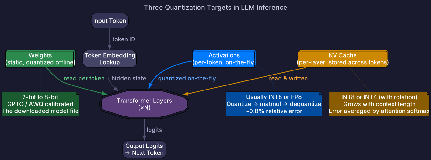
Weights are fixed after training and quantized once offline — this is where the most aggressive compression happens (2-bit to 8-bit), calibrated with methods like GPTQ or AWQ. This is literally the downloaded model file.

Activations change with every input and must be quantized on-the-fly during the forward pass — usually to INT8 or FP8. The quantize → matmul → dequantize cycle adds ~0.8% relative error.

The KV cache stores Key and Value vectors for every token across all attention layers. It grows linearly with context length and can be quantized to INT8 or INT4 (with rotation techniques). The error is naturally averaged by the attention softmax. For more on why KV cache memory dominates inference costs, see The KV Cache Problem — Why Memory Is the New Compute.

---

Technique Deep Dive: Weight Quantization

Weights are fixed after training and quantized once. This is where the most aggressive compression happens.

Naive Round-to-Nearest vs. Calibrated Quantization

The simplest approach — round each weight to the nearest quantized value — leaves quality on the table. Modern methods are much smarter.

GPTQ applies Optimal Brain Quantization layer by layer. It quantizes one weight column at a time and uses the inverse Hessian (computed from a small calibration dataset, typically 128 samples) to adjust the remaining unquantized weights, compensating for the error just introduced:

For each column j in the weight matrix W:
    1. Quantize column j:  w_q[j] = round(w[j] / scale) × scale
    2. Compute the error:  δ = w[j] - w_q[j]
    3. Compensate remaining columns using the Hessian:
       w[j+1:] += δ × H_inv[j, j+1:] / H_inv[j, j]

This takes minutes on a single GPU and produces measurably better results than naive rounding — typically 0.1-0.3 perplexity points better at 4-bit.

AWQ (Activation-Aware Weight Quantization) takes a different approach. It observes that a small fraction of weight channels (~1%) correspond to large activation magnitudes, and these channels disproportionately affect quality. By scaling salient weights up before quantization (and scaling activations down to compensate), the important weights get more effective precision within the same bit budget.

What the numbers actually look like

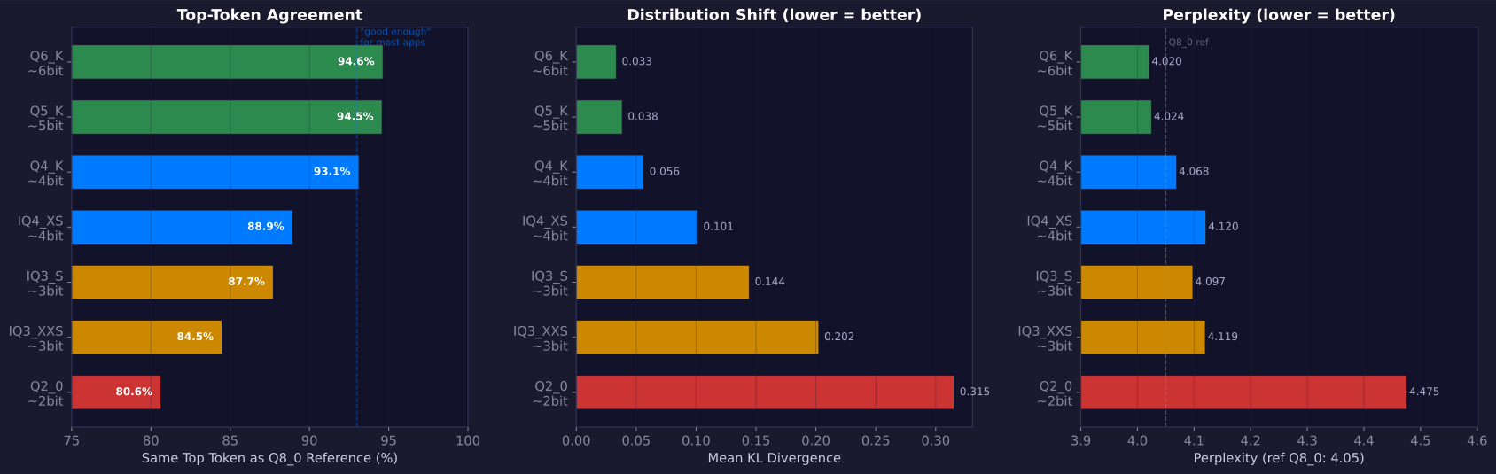
Here’s measured data from a 70B+ MoE model, scored against a Q8_0 reference on a fixed evaluation set of ~5,000 tokens across code, prose, and multilingual text:

Key observations:

• Q4_K (4-bit) agrees with Q8_0 on the most-likely token 93% of the time. For most applications, this is indistinguishable.
• Even Q2_0 (2-bit) agrees 80% of the time. The perplexity increase is ~10%, which is significant but still usable.
• The quality degradation is smooth and predictable — there’s no cliff. You can choose your tradeoff point.

Memory savings at each level

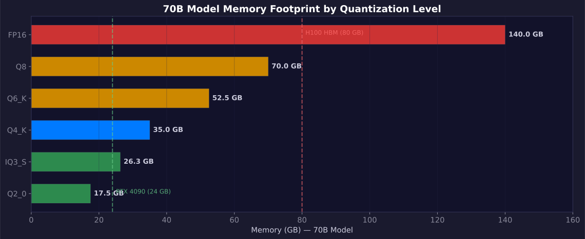
The practical impact is dramatic: at Q4_K, a 70B model fits in 35 GB — within reach of a single GPU or a high-end laptop with unified memory. At Q2_0, it fits in 17.5 GB — on a consumer RTX 4060 Ti.

---

Technique Deep Dive: Activation Quantization

Activations are the intermediate values flowing through the network. Unlike weights, they change with every input and must be quantized on-the-fly during the forward pass.

Why quantize activations at all?

When you do a matrix multiply Y = X × W, both operands travel from memory to the compute units. Quantizing only the weights saves half the bandwidth. Quantizing both (e.g., INT8 activations × INT4 weights) saves more, and critically, enables integer tensor core operations that run at 2× the throughput of FP16.

The precision subtleties matter

This is where practical experience diverges from textbook descriptions. In real inference engines, numerical consistency is paramount — especially when the same computation can happen on different hardware paths (GPU for “hot” data, CPU for “cold” data in MoE models):

1. The scale is computed in FP32 but stored as FP16. The quantized integers are computed by dividing by the FP32 scale, but the dequantized value multiplies by the FP16 scale. Mixing these up shifts values at every rounding boundary.

2. The rounding rule must be consistent. GPU paths may use rint (round half to even), while CPU paths use round (round half away from zero). These differ at exactly 0.5 boundaries.

3. FP64 intermediate precision is used in careful implementations for the quantization step itself. The division x[i] / d in FP32 has different rounding from FP64, and this matters when the quotient is near 0.5.

These details are invisible in papers but critical in production code.

---

Technique Deep Dive: KV Cache Quantization

The KV cache stores Key and Value vectors for every token in the context, at every attention layer. For long-context inference, this dominates memory — a 70B model at 128K context uses ~40 GB just for KV cache in FP16. (See our deep dive on KV cache economics for why this is the #1 constraint in serving.)

INT8 KV Cache: The Simple Case

Quantizing K and V to INT8 as they’re written follows the same block quantization as activations. Each group of 64 elements gets its own FP16 scale — straightforward and nearly lossless.

INT4 KV Cache: Walsh-Hadamard Rotation

Going to 4-bit is much more aggressive — only 16 distinct levels per value. Naive Q4 on the KV cache produces visible quality loss. The solution is an orthogonal rotation before quantizing.

The Walsh-Hadamard Transform (WHT) spreads each element’s information across all dimensions. Before WHT, raw K vectors have outliers — a few elements 10× larger than the rest eat the entire block’s dynamic range. After WHT, outlier energy is spread evenly, making all 16 quantization levels used efficiently.

The WHT is computed on GPU using warp-level __shfl_xor operations — a butterfly network costing only ~log₂(256) = 8 add/subtract operations per element. Nearly free. The mathematical insight from QuIP#: an orthogonal rotation makes the quantization error isotropic (equal in all directions), which is provably optimal for a uniform quantizer.

---

The Error Budget: Why It All Works Together

The natural concern: if you’re quantizing weights, activations, and the KV cache, don’t the errors compound through 80+ layers and produce garbage?

In practice, no.

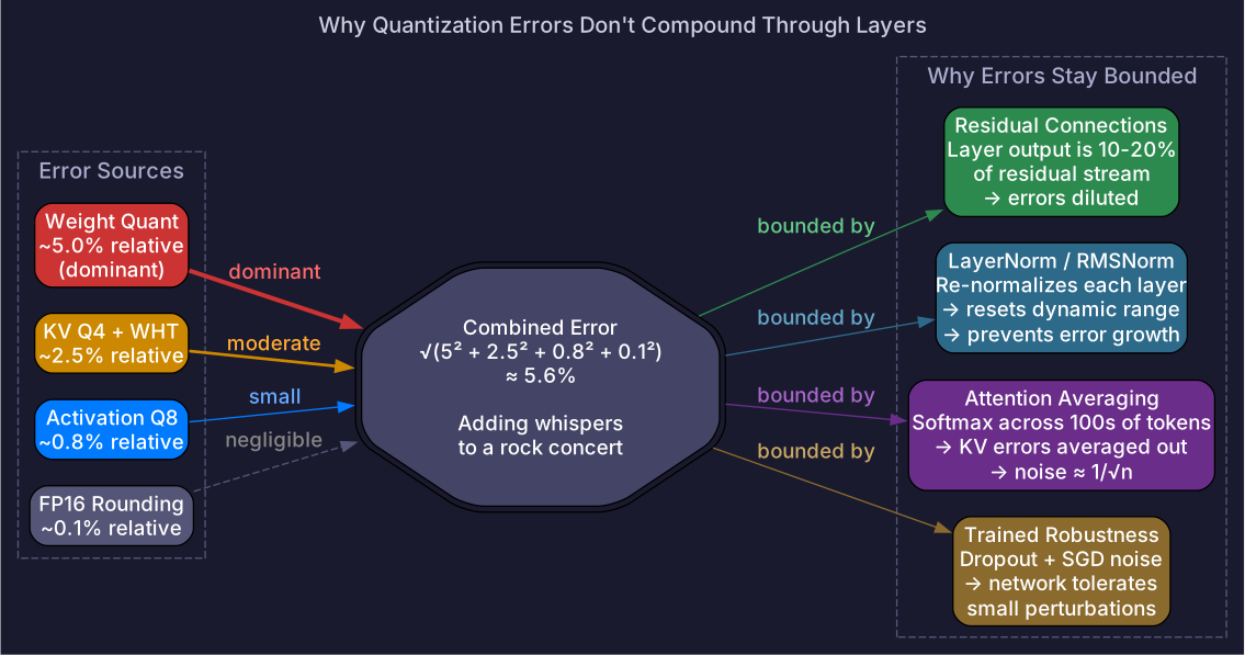
The different sources of quantization noise are not equal, and the dominant source sets the floor. Weight quantization at ~5% relative error dwarfs activation quantization at ~0.8%. Adding activation error on top: √(5.0² + 0.8²) = 5.06% — barely changes the total. It’s like adding a whisper to a rock concert.

Why errors don’t compound exponentially through layers:

1. Residual connections. Every transformer layer adds its output to the input. The layer’s contribution is typically 10-20% of the residual stream magnitude, so errors are diluted.

2. LayerNorm / RMSNorm. Each layer re-normalizes its input, preventing error growth — it’s essentially a dynamic range reset every layer.

3. Attention is averaging. Softmax distributes weight across hundreds of tokens. Individual KV cache quantization errors are averaged out (noise ≈ 1/√n).

4. Trained robustness. Models are trained with dropout, noise, and SGD stochasticity. They’ve never seen “exact” inputs, even during training.

---

Quantization Formats: The Zoo

Not all quantization is just “round to the nearest integer.” The format determines both quality and kernel complexity.

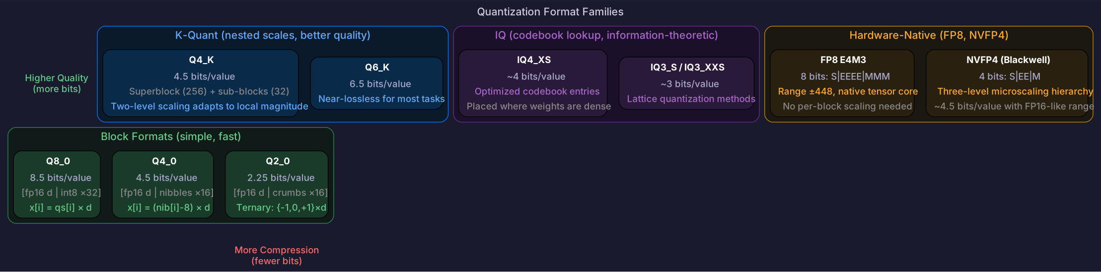
Block Formats (Q8_0, Q4_0, Q2_0)

Simple symmetric quantization with a single scale per block. Fast to compute, easy to implement. The workhorse of inference engines.

K-Quant: Nested Scales for Better Dynamic Range

K-quants use a two-level scaling structure: a superblock of 256 values contains sub-blocks of 16-32 values, each with its own fine-grained scale. Different regions of a weight vector may have very different magnitudes — per-sub-block scales adapt to local magnitude, giving better quality at the same bit budget.

IQ (Information-Theoretic) Quantization

Instead of uniformly spaced quantization levels, IQ formats use optimized codebooks — lookup tables whose entries are chosen to minimize expected quantization error. The codebook entries cluster where the weight distribution is densest, giving more precision where it matters. IQ2_XS uses just 2 bits per weight with lattice quantization methods.

FP8 and NVFP4: Hardware-Native Formats

FP8 E4M3 (8 bits: Sign + 4 exponent + 3 mantissa) handles varying magnitudes without per-block scaling — the exponent provides 16× dynamic range natively. Supported by Hopper tensor cores at 2× FP16 throughput.

NVFP4 (Blackwell) uses a three-level microscaling hierarchy: per-tensor FP32 global scale → per-16-value UE8M0 block scale → per-4-value UE4M3 sub-block scale → per-value E2M1. Effective: ~4.5 bits/value with FP16-like range.

---

Where Quantization Lives in the Inference Pipeline

Here’s how a single token decode step flows through a quantized inference engine, with the quantization points marked:

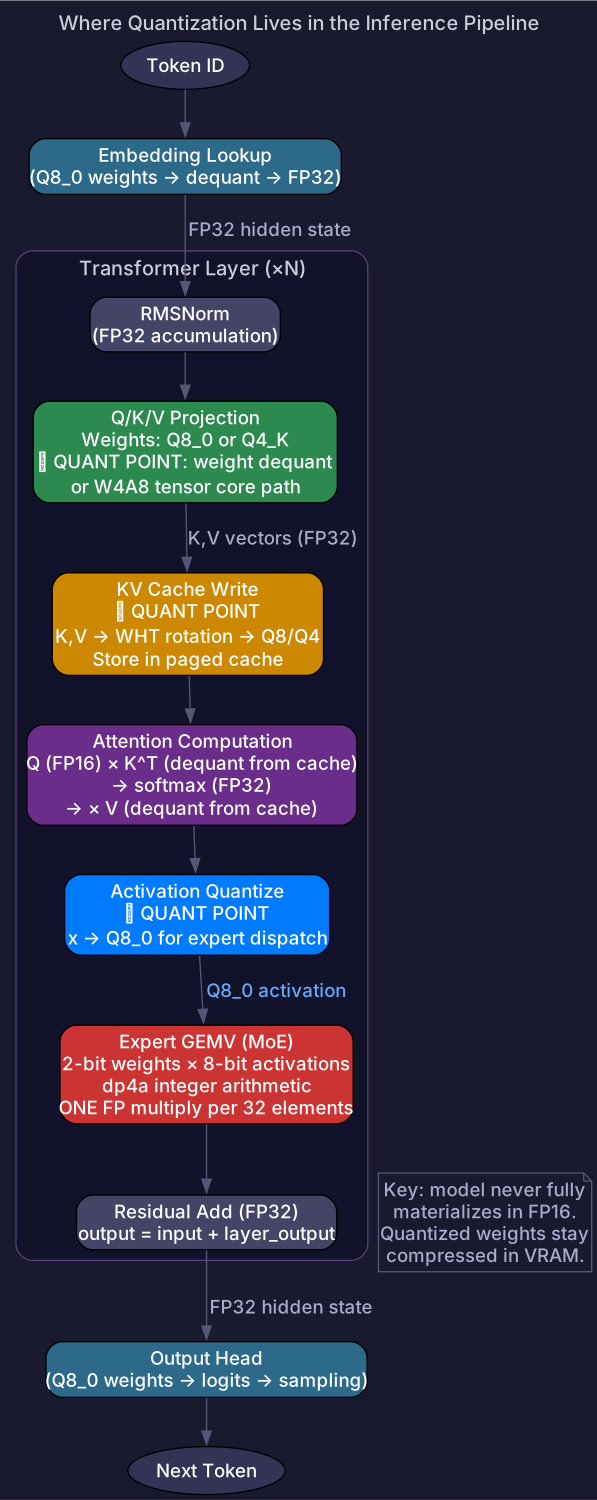
Key observation: the model never fully materializes in FP16. Quantized weights stay compressed in VRAM. Each operation dequantizes a small tile just before use (fused into the GEMM kernel), or computes directly in the quantized domain via dp4a integer instructions.

The dp4a Trick: Integer Arithmetic in the Inner Loop

The dp4a (dot product of 4 × int8, accumulated in int32) instruction is what makes quantized compute practical. One instruction replaces 4 multiply-accumulates in FP32:

dp4a operation (one CUDA instruction):

  a = [a₃, a₂, a₁, a₀]   ← 4 × int8 packed in one int32
  b = [b₃, b₂, b₁, b₀]   ← 4 × int8 packed in one int32

  result = c + a₀×b₀ + a₁×b₁ + a₂×b₂ + a₃×b₃

  All integer, exact (no rounding), one clock cycle.

In the 2-bit weight × 8-bit activation inner loop, the FP multiply that dominates FP16 GEMV is replaced by integer dp4a + one FP multiply per block of 32 elements. This is why quantized inference is fast — and why understanding the prefill vs decode split matters for choosing the right quantization strategy.

---

MoE Models: Where Quantization Gets Interesting

Mixture-of-Experts models like DeepSeek-V3 (671B total, ~37B active) introduce a unique interaction between quantization and memory management.

Quantization Enables the Memory Hierarchy

A 166B MoE model has ~24,000 expert sub-networks. On a 12 GB GPU, only a fraction can be resident in VRAM at once:

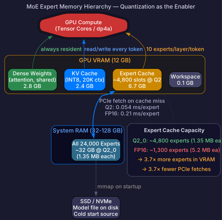
Without quantization, each expert at FP16 would be ~5.2 MB — the same VRAM cache holds only ~1,300 experts. At Q2_0 (1.35 MB per expert), you get 3.7× more experts resident in VRAM, dramatically improving cache hit rates.

Quantization also makes paging viable: fetching a Q2_0 expert over PCIe takes 0.054 ms vs 0.21 ms for FP16. With 10 cache misses per token, that’s 0.54 ms vs 2.1 ms — the difference between hitting and missing a 20 tok/s budget.

Activation Quantization Saves PCIe Bandwidth

When experts live in CPU RAM, quantizing activations to Q8 before the PCIe transfer halves the bandwidth: 2.72 KB round trip instead of 10 KB — a 3.3× reduction per expert dispatch.

---

Practical Impact: Real Numbers

Speed (tokens per second)

On consumer hardware running a 166B MoE model with 2-bit experts:

Decode speed (tokens/s) by hardware:

  RTX 5070 12GB, 64GB RAM
  ████████████████████████████████████████  ~20 tok/s

  RTX 3060 12GB, 46GB RAM
  ████████████████████████████  ~14 tok/s

  Apple M5 Max, 128GB unified
  ████████████████████████████████████  ~18 tok/s

  4× Radeon AI PRO R9700
  ████████████████████████████████████████████████████████████  55-69 tok/s
  (with speculative decoding)

  These are 166B parameter models running on $300–$2,000 hardware,
  not $30,000 H100s.

Memory-Bandwidth Arithmetic

Why quantization translates directly to speed for token generation:

Token generation is memory-bandwidth bound (batch=1):

  Model     Format    Bytes to read    Time @ 1 TB/s    Tokens/s
  ─────     ──────    ─────────────    ─────────────    ────────
  70B       FP16      140 GB           140 ms            7.1
  70B       Q8        70 GB            70 ms             14.3
  70B       Q4        35 GB            35 ms             28.6

  Quantization speedup ≈ compression ratio (for decode)

This is why 4-bit is ~4× faster than FP16, not ~2× — and why understanding the attention bottleneck matters for the full picture.

---

The Future: Where Quantization Is Heading

The physical world can’t wait for the cloud

2026 has made one thing clear: LLMs are no longer just chatbots. GPT-6 Astra understands physical space. Google’s Gemini 4 processes continuous video streams with spatial awareness. These models don’t just generate text — they perceive, reason about, and act in the physical world.

This changes the quantization conversation entirely.

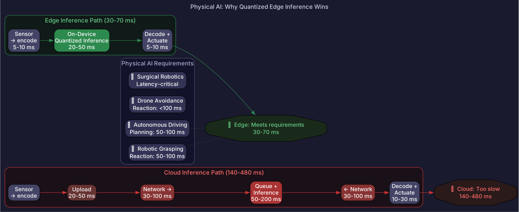
When an LLM powers a chat interface, 200ms of latency is fine. But when that same model controls a robotic arm, navigates an autonomous vehicle, or guides a surgical instrument, 200ms is the difference between success and catastrophe.

The implication is stark: if you want frontier AI capabilities in the physical world, you need frontier models running on edge hardware. A 2-bit quantized 70B VLM fits in 18 GB — within reach of a Jetson AGX Orin (64 GB), a Snapdragon X Elite (32 GB), or even a single RTX GPU.

This isn’t hypothetical:

• Humanoid robots (Figure, Tesla Optimus, 1X) need multimodal reasoning for manipulation tasks
• Autonomous vehicles run vision-language models for scene understanding — the model must run on the vehicle, not in a data center 500 miles away
• Industrial robots in factories where network outages happen — a robot that stops when WiFi drops is not acceptable
• Medical devices where patient data cannot leave the device for regulatory reasons

Hardware-native sub-8-bit compute

Blackwell’s FP4 tensor cores and AMD’s planned INT4 MFMA instructions signal that sub-8-bit compute is becoming a first-class hardware feature. The W4A4 path — 4-bit weights × 4-bit activations — already exists in experimental kernels.

Training-aware quantization

BitNet shows that models trained natively in 1.58-bit (ternary: {-1, 0, 1}) can match FP16 quality — eliminating floating-point multiply entirely. If this scales, purpose-built chips for ternary matrix operations would be dramatically simpler and more power-efficient than GPUs.

The convergence

The most important trend isn’t any single technique — it’s the convergence of model design, quantization methods, and edge hardware into a co-designed stack. MoE architectures are inherently quantization-friendly for edge. Apple’s recent silicon puts 192-512 GB of unified memory on a single chip. NVIDIA’s Jetson Thor targets humanoid robots with INT4/FP8 tensor cores.

The trajectory:

  2023 │ Quantization = "make it fit" (a compression trick)
  2024 │ Quantization = "make it fast" (a bandwidth optimization)
  2025 │ Quantization = "make it run anywhere" (edge deployment)
  2026 │ Quantization = "make it real" (physical AI, embodied agents)
  2027+│ Quantization = invisible infrastructure
       │ (co-designed with model architecture and silicon)

---

Practical Advice: Getting Started

1. Start with FP8 if you have Hopper/Blackwell hardware. Nearly lossless, no calibration needed, natively supported by tensor cores.

2. Use GPTQ or AWQ for 4-bit weight quantization when fitting a model on fewer GPUs. Q4_K agrees with Q8_0 on 93% of top-token predictions.

3. Quantize the KV cache to INT8 for long-context workloads. For INT4 KV, use Hadamard rotation — mathematically proven optimal and computationally nearly free.

4. Profile before optimizing. Measure whether your workload is memory-bandwidth bound (token generation) or compute-bound (prompt processing). Quantization helps the former dramatically. For the latter, use lower-precision tensor core formats (FP8, INT8).

5. Always validate end-to-end on your actual task. Perplexity is a proxy. The right tradeoff point varies by domain — code generation is more sensitive than open-ended chat.

6. For MoE models, think about the memory hierarchy. Quantization determines not just memory needs, but how many experts fit in your VRAM cache and how fast cache misses resolve over PCIe.

---

Conclusion

Quantization is not a hack or a shortcut. It’s an engineering discipline that trades unnecessary numerical precision for the resources that actually matter — memory capacity, memory bandwidth, power efficiency, and increasingly, the ability to deploy intelligence at the point of action.

The key insights:

• Weight quantization is done offline with calibration. It’s the biggest compression lever and the dominant source of quality loss.
• Activation and KV cache quantization happen on-the-fly. They add negligible error on top of weight quantization.
• The errors don’t compound thanks to residual connections, normalization layers, and the averaging nature of attention.
• Quantization is a bandwidth optimization, not just a storage trick. Smaller data types = less memory traffic = directly faster inference.
• For MoE models, quantization enables an entire memory hierarchy that makes 100B+ models runnable on consumer hardware.
• For physical AI, quantization is the enabling technology — the bridge between frontier model capability and the constraints of the real world.

We’re entering an era where the most capable AI models won’t just live in data centers. They’ll be in warehouses, operating rooms, vehicles, and homes. Every one of those deployments will run a quantized model, because the physics of networks and the physics of the real world leave no alternative.

---

References

1. Frantar, E., et al. (2022). GPTQ: Accurate Post-Training Quantization for Generative Pre-trained Transformers. arXiv:2210.17323.
2. Lin, J., et al. (2023). AWQ: Activation-Aware Weight Quantization for LLM Compression and Acceleration. arXiv:2306.00978.
3. Chee, J., et al. (2024). QuIP#: Even Better LLM Quantization with Hadamard Incoherence and Lattice Codebooks. arXiv:2402.04396.
4. Xiao, G., et al. (2023). SmoothQuant: Accurate and Efficient Post-Training Quantization for Large Language Models. arXiv:2211.10438.
5. Ma, S., et al. (2024). The Era of 1-bit LLMs: All Large Language Models are in 1.58 Bits. arXiv:2402.17764.
6. Dettmers, T., et al. (2022). LLM.int8(): 8-bit Matrix Multiplication for Transformers at Scale. arXiv:2208.07339.
7. Shao, W., et al. (2024). OmniQuant: Omnidirectionally Calibrated Quantization for Large Language Models. arXiv:2308.13137.