Build GPT from Scratch in 500 Lines of PyTorch

TL;DR

We build a working GPT from scratch — tokenizer, transformer, pretraining, fine-tuning, and inference with KV cache — in ~500 lines of PyTorch on a MacBook. The model is tiny (3.3M params, trains in 1 minute) but uses the exact same architecture as GPT-4. Key takeaways: (1) BPE tokenization is just compression — frequent byte pairs merge into tokens. (2) Self-attention lets every token dynamically attend to all previous tokens; the causal mask is what makes it generative. (3) Pretraining’s only objective is next-token prediction — grammar, facts, and reasoning emerge as side effects. (4) Fine-tuning changes behavior (answer questions vs. continue text) without changing the architecture or loss function. (5) KV cache turns inference from O(n²) to O(n) by caching past Keys/Values. Written for infra and software engineers who work around AI daily but want to understand what’s actually inside the black box.

---

If you work in infrastructure — whether that’s ML platforms, serving systems, or capacity planning — you hear terms like “transformer”, “attention”, “KV cache”, and “tokenizer” every day. You provision GPUs for them, optimize latency around them, and debug serving failures caused by them. But what do they actually do?

This guide builds a complete GPT language model from scratch in ~500 lines of PyTorch, running entirely on a MacBook. Same decoder-only transformer architecture as GPT-2/3/4 — just smaller. No distributed training, no cloud GPUs, no pre-built libraries. Just PyTorch and first principles.

The goal isn’t to train a production model. It’s to give engineers who work around AI a first-hand understanding of what’s happening inside the black box — so the next time you’re debugging a CUDA OOM, tuning batch sizes for a serving fleet, or sizing KV cache memory, you know exactly what those numbers map to in the model.

The build follows the real-world order: get data → tokenize → build model → pretrain → fine-tune → run inference. All code is open-source at github.com/the-last-programmers/gpt-from-scratch.

---

Table of Contents

1. What Is GPT
2. Data + Tokenization
3. The Transformer Architecture
4. Pretraining
5. Fine-tuning
6. Inference

---

1. What Is GPT

Why Build from Scratch?

Everyone uses ChatGPT. Very few people understand what’s actually happening inside — including many engineers who build the infrastructure that runs it.

As a software engineer or infra engineer, you probably know these terms at a high level: attention, embeddings, tokens, next-token prediction. But there’s a gap between “I’ve read the Wikipedia summary” and “I understand why the KV cache saves O(n) compute per generated token.” Building the thing yourself — even a tiny version — closes that gap permanently.

This guide is written for that audience: engineers who are technical but not ML researchers. Every concept is explained from first principles, paired with working code. By the end, you’ll have a working model that generates text and follows instructions, running entirely on your laptop.

GPT = Generative Pre-trained Transformer

• Generative: it produces text one token at a time, left to right
• Pre-trained: it learns language structure from a massive text corpus before being specialized
• Transformer: the neural network architecture it’s built on (introduced in “Attention Is All You Need”, 2017)

GPT is a decoder-only transformer:

• It only looks backward — each token can attend to all previous tokens, never future ones
• It generates autoregressively — predicting one token at a time, feeding each prediction back as input
• There is no separate “encoder” — unlike models like BERT or T5

This is the same architecture behind GPT-2, GPT-3, GPT-4, Claude, and most modern large language models.

The Full Architecture at a Glance

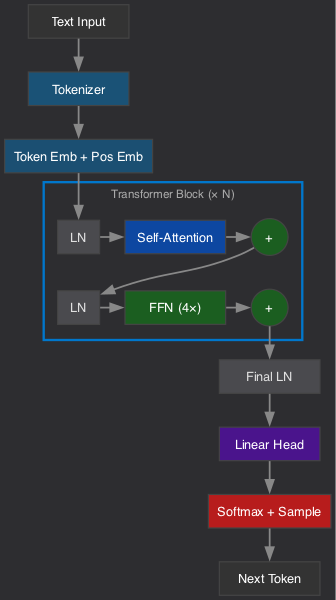
Component	What It Does	Why It Exists
Tokenizer	Splits text into subword pieces	Models need fixed-vocabulary integers, not arbitrary strings
Token Embedding	Maps each token ID to a vector	Gives the model a learnable representation of each token
Position Embedding	Encodes where each token sits in the sequence	Transformers have no built-in sense of order
Causal Self-Attention	Lets each token attend to all previous tokens	The mechanism for understanding context
Feed-Forward Network	Per-token nonlinear transformation	Adds capacity — most of the model’s parameters live here
Residual Connections	Skip connections around each sub-layer	Allows training deep networks without vanishing gradients
LayerNorm	Normalizes activations	Stabilizes training
Linear Head	Projects from embed_dim to vocab_size	Produces a probability distribution over next tokens

The Build Order

We follow the real-world order — the way you’d actually build this if you sat down on a weekend:

1. Data + Tokenization — Get text, convert it to numbers the model can process
2. Model Architecture — Build the transformer: embeddings, attention, feed-forward blocks
3. Pretraining — Train the model to predict the next token
4. Fine-tuning — Teach it to follow instructions instead of just continuing text
5. Inference — Run it: generate text with KV cache and sampling strategies

What We’re NOT Building

To keep this tractable and educational:

• No distributed training (single machine, single device)
• No Flash Attention (same math, just an optimization)
• No RLHF (we do supervised fine-tuning only)
• No rotary position embeddings (we use learned positional, like GPT-2)
• No mixture of experts

These are all important at scale. But the core mechanism — the thing that makes a transformer work — doesn’t need any of them.

Requirements

• Python 3.10+
• PyTorch 2.0+
• A Mac with Apple Silicon (MPS backend) — or any machine with a CPU
• ~10 minutes of patience for training

pip install torch
git clone https://github.com/the-last-programmers/gpt-from-scratch
cd gpt-from-scratch
python run.py

The entire pipeline runs end-to-end with one command.

---

2. Data + Tokenization

Neural networks need numbers, not text. Byte Pair Encoding (BPE) solves this by iteratively merging the most frequent character pairs into tokens — a compression algorithm repurposed for NLP. It hits the sweet spot between word-level (vocabulary too large) and character-level (sequences too long).

The Problem

Neural networks operate on numbers. They can’t process the string "Hello, world!" directly. We need a way to convert arbitrary text into a sequence of integers from a fixed vocabulary — and convert back.

This is tokenization, and it’s the first decision that shapes everything downstream:

• Too few tokens (word-level): the vocabulary explodes. Millions of unique words, most appearing rarely. The embedding table becomes enormous and most entries barely get trained.
• Too many tokens (character-level): sequences become very long. Attention is O(n²) — doubling sequence length quadruples compute cost.
• The sweet spot (subword-level): common words are single tokens, rare words split into recognizable pieces. This is what all modern LLMs use.

Byte Pair Encoding (BPE)

BPE is the algorithm behind GPT’s tokenizer. It was originally a compression algorithm (1994), repurposed for NLP.

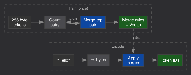
Training the tokenizer:

1. Start with 256 base tokens (one per byte value — covers all UTF-8 text)
2. Scan the corpus. Count every adjacent pair of tokens.
3. Find the most frequent pair. Merge it into one new token.
4. Repeat until you reach your desired vocabulary size.

Using the tokenizer (encoding):

1. Convert text to bytes
2. Apply the learned merges in order (lowest merge first)
3. Output: a sequence of token IDs

Concrete example:

Corpus: "low lower lowest"

Step 1: Start as bytes
  ['l','o','w',' ','l','o','w','e','r',' ','l','o','w','e','s','t']

Step 2: Most frequent pair? ('l','o') appears 3 times
  → Merge into token 256: "lo"
  ['lo','w',' ','lo','w','e','r',' ','lo','w','e','s','t']

Step 3: Most frequent pair? ('lo','w') appears 3 times
  → Merge into token 257: "low"
  ['low',' ','low','e','r',' ','low','e','s','t']

Step 4: Most frequent pair? ('low','e') appears 2 times
  → Merge into token 258: "lowe"
  ['lowe','r',' ','lowe','s','t',' ','low']

...and so on until we hit vocab_size.

The result: common words compress into single tokens. Rare words gracefully decompose into subword pieces. The system never hits an “unknown token” — it can always fall back to raw bytes.

Why BPE and Not Something Else?

Approach	Pros	Cons
Word-level	Semantically meaningful	Huge vocab, can’t handle typos/new words
Character-level	Small vocab, handles anything	Sequences too long, attention too expensive
BPE	Balanced vocab, handles everything, compresses well	Merges are greedy, not globally optimal
WordPiece	Similar to BPE	Uses likelihood instead of frequency — slightly better but harder to implement
Unigram	Globally optimal subword selection	More complex, less intuitive

GPT-2/3/4 all use BPE. It’s simple, effective, and fast enough.

Implementation: Training the Merges

def train(self, text, vocab_size=512):
    # Split text into words using a regex pattern
    # This prevents merges across word boundaries
    words = self.pattern.findall(text)

    # Convert each word to a list of byte values
    # "Hello" → [72, 101, 108, 108, 111]
    token_sequences = [list(word.encode("utf-8")) for word in words]

    # Start with 256 byte-level tokens
    self.vocab = {i: bytes([i]) for i in range(256)}
    next_token = 256

    # Iteratively merge the most common pair
    while next_token < vocab_size:
        # Count every adjacent pair across all sequences
        pair_counts = self._get_pair_counts(token_sequences)
        if not pair_counts:
            break

        # The most frequent pair becomes our next token
        best_pair = max(pair_counts, key=pair_counts.get)

        # Replace every occurrence of this pair with the new token
        token_sequences = self._merge_pair(
            token_sequences, best_pair, next_token
        )

        # Record the merge rule and the new token's bytes
        self.merges[best_pair] = next_token
        self.vocab[next_token] = self.vocab[best_pair[0]] + self.vocab[best_pair[1]]
        next_token += 1

Why the regex pattern? We split on word boundaries before counting pairs. Without this, BPE would merge across words — “the end” might produce a “e e” token that spans two words, which is linguistically nonsensical and hurts downstream performance. GPT-2’s original regex:

pattern = r"""'s|'t|'re|'ve|'m|'ll|'d| ?\w+| ?\d+| ?[^\s\w]+|\s+"""

Implementation: Encoding (Applying Merges)

def encode(self, text):
    words = self.pattern.findall(text)
    token_ids = []

    for word in words:
        # Start with raw bytes
        tokens = list(word.encode("utf-8"))

        # Apply merges in priority order (lowest merge ID first)
        while len(tokens) >= 2:
            # Find which mergeable pairs exist in this sequence
            pair_counts = {}
            for i in range(len(tokens) - 1):
                pair = (tokens[i], tokens[i + 1])
                if pair in self.merges:
                    pair_counts[pair] = self.merges[pair]

            if not pair_counts:
                break

            # Apply the EARLIEST merge (lowest ID = most frequent in training)
            best_pair = min(pair_counts, key=pair_counts.get)
            new_token = self.merges[best_pair]

            # Merge all occurrences of this pair
            new_tokens = []
            i = 0
            while i < len(tokens):
                if i < len(tokens) - 1 and (tokens[i], tokens[i + 1]) == best_pair:
                    new_tokens.append(new_token)
                    i += 2
                else:
                    new_tokens.append(tokens[i])
                    i += 1
            tokens = new_tokens

        token_ids.extend(tokens)

    return token_ids

Why apply merges in priority order? The merge with the lowest ID was learned first — meaning it was the most frequent pair in training. Applying merges in this order ensures consistent tokenization: the same text always produces the same tokens.

Implementation: Decoding

def decode(self, token_ids):
    byte_seq = b"".join(self.vocab[t] for t in token_ids)
    return byte_seq.decode("utf-8", errors="replace")

Decoding is trivial: each token ID maps to a byte sequence. Concatenate them all and decode as UTF-8.

Running It

python download_data.py    # Get training corpus
python tokenizer.py        # Train BPE tokenizer

Output:

Trained tokenizer: 512 tokens
Original:  Hello, world! This is a test.
Encoded:   [72, 455, 111, 44, 464, 316, 33, 508, 104, 271, 360, 258, 256, 412, 46]
Decoded:   Hello, world! This is a test.

The Training Data

We use public domain books from Project Gutenberg plus Shakespeare — about 5.7MB total, roughly 2.7 million tokens after BPE encoding. Tiny by modern standards (GPT-3 was trained on 300 billion tokens), but sufficient to learn basic English structure.

The choice of training data matters:

• Train on code → the tokenizer creates tokens like def, return, self.
• Train on English prose → tokens like the, tion, ing
• Train on mixed data → balanced subwords that handle both

Key Takeaways

1. Tokenization is compression. BPE finds the most efficient encoding of your corpus given a fixed vocabulary size.
2. The vocab_size is a fundamental tradeoff. Larger = shorter sequences (cheaper attention) but larger embedding table. GPT-2 uses 50K. Our toy model uses 512.
3. BPE guarantees no unknown tokens. It can always fall back to individual bytes.
4. Tokenization is separate from the model. The tokenizer is trained once and frozen.

---

3. The Transformer Architecture

The GPT architecture is a stack of transformer blocks, each containing causal self-attention (lets each token attend to all previous tokens) and a feed-forward network (per-token nonlinear processing). The entire model is ~200 lines of Python.

The Problem

We have a sequence of token IDs. We need a function that takes those IDs and outputs a probability distribution over what token comes next. The transformer is that function.

The challenge: language has long-range dependencies. The word “it” in sentence 50 might refer to something mentioned in sentence 3. The model needs a mechanism to let any token attend to any previous token — regardless of distance. This is what self-attention provides.

The Big Picture

Step 1: Embeddings — Giving Tokens Meaning

A token ID like 372 is meaningless to a neural network. We need to map it to a dense vector that the model can learn with.

self.token_emb = nn.Embedding(vocab_size, embed_dim)    # 512 × 256
self.pos_emb = nn.Embedding(context_length, embed_dim)  # 128 × 256

Token embedding: a lookup table. Token 372 → row 372 of a [vocab_size × embed_dim] matrix. Each row is initialized randomly and trained via backpropagation. After training, tokens with similar meanings end up with similar vectors.

Position embedding: transformers process all tokens in parallel (unlike RNNs which go left-to-right). Without position information, “the cat sat on the mat” and “mat the on sat cat the” would produce identical representations. Position embedding adds a learnable vector for each position (0, 1, 2, …) so the model knows token order.

def forward(self, idx):
    B, T = idx.shape

    # Position indices: [0, 1, 2, ..., T-1]
    pos = torch.arange(0, T, device=idx.device).unsqueeze(0)

    # Look up embeddings and add them together
    tok_emb = self.token_emb(idx)   # [B, T, embed_dim]
    pos_emb = self.pos_emb(pos)     # [1, T, embed_dim] — broadcasts over batch
    x = tok_emb + pos_emb           # [B, T, embed_dim]

Why addition and not concatenation? Concatenation would double the dimension (wasting half the model’s capacity on position info). Addition works because the model learns to use orthogonal subspaces for positional and semantic information — they don’t interfere much in practice.

Step 2: Causal Self-Attention — The Core Mechanism

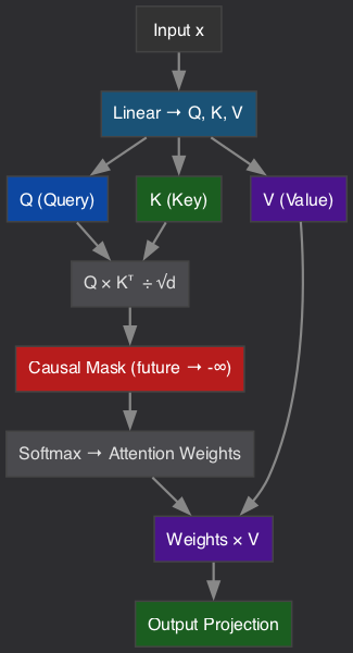
This is the heart of the transformer. Self-attention lets each token look at every previous token and decide which ones are relevant for predicting the next word.

The Intuition

Think of reading a sentence:

“The cat, who was very old and tired, finally sat on the mat.”

When processing “sat”, the model needs to know:

• WHO sat? → attend to “cat” (far away)
• Ignore the relative clause → low attention to “who was very old and tired”

Self-attention computes this relevance dynamically for every token pair.

Query, Key, Value

The mechanism uses three projections of the same input:

• Query (Q): “What am I looking for?” — what information this token needs
• Key (K): “What do I contain?” — what information this token offers
• Value (V): “What do I actually provide?” — the content to pass forward if selected

# Single linear layer produces all three: Q, K, V
self.qkv = nn.Linear(embed_dim, 3 * embed_dim)

# Split into Q, K, V
qkv = self.qkv(x)                    # [B, T, 3 * embed_dim]
q, k, v = qkv.split(embed_dim, dim=-1)  # each [B, T, embed_dim]

Why one combined linear layer? Efficiency. Three separate layers would do the same math but with three separate matrix multiplications. One combined layer followed by a split is faster on GPUs.

Computing Attention Scores

# Reshape for multi-head: [B, T, embed_dim] → [B, n_heads, T, head_dim]
q = q.view(B, T, n_heads, head_dim).transpose(1, 2)
k = k.view(B, T, n_heads, head_dim).transpose(1, 2)
v = v.view(B, T, n_heads, head_dim).transpose(1, 2)

# Dot product between queries and keys
# Each q[i] asks: "how relevant is k[j] to me?"
attn = (q @ k.transpose(-2, -1)) * (head_dim ** -0.5)

Why scale by 1/√(head_dim)? Without scaling, the dot products grow with dimension size. Large dot products push softmax into regions where gradients are tiny (near 0 or 1), making learning slow. Scaling keeps the variance stable regardless of dimension.

The Causal Mask — What Makes It “Decoder-Only”

# Lower-triangular matrix: 1s below diagonal, 0s above
mask = torch.tril(torch.ones(context_length, context_length))

# Example for seq_len=5:
# [[1, 0, 0, 0, 0],   ← token 0 sees only itself
#  [1, 1, 0, 0, 0],   ← token 1 sees tokens 0-1
#  [1, 1, 1, 0, 0],   ← token 2 sees tokens 0-2
#  [1, 1, 1, 1, 0],   ← token 3 sees tokens 0-3
#  [1, 1, 1, 1, 1]]   ← token 4 sees all previous

# Set masked positions to -infinity (softmax → 0 probability)
attn = attn.masked_fill(mask[:T, :T] == 0, float("-inf"))

This is the critical constraint. By masking future tokens, we guarantee:

1. The model can never “cheat” by looking ahead during training
2. Each position’s prediction depends only on past context
3. The model can generate text left-to-right at inference time

Without this mask, it’s a BERT-style encoder (bidirectional). With it, it’s GPT (autoregressive).

Softmax and Output

# Convert scores to probabilities (each row sums to 1)
attn = F.softmax(attn, dim=-1)
attn = self.attn_dropout(attn)

# Weighted sum of values — high-attention tokens contribute more
out = attn @ v  # [B, n_heads, T, head_dim]

# Reshape back: [B, n_heads, T, head_dim] → [B, T, embed_dim]
out = out.transpose(1, 2).contiguous().view(B, T, embed_dim)

# Final projection
return self.out_proj(out)

Multi-Head Attention — Why Multiple Heads?

Instead of one big attention computation, we split into N smaller ones (heads), each operating on embed_dim / n_heads dimensions.

Why? Different heads learn different patterns:

• Head 1 might learn syntactic relationships (subject-verb agreement)
• Head 2 might learn coreference (“she” → “Alice”)
• Head 3 might learn positional patterns (adjacent words)
• Head 4 might learn semantic similarity

With one head, these patterns would interfere. Multiple heads let the model track multiple relationships simultaneously, then combine them via the output projection.

embed_dim = 256, n_heads = 4 → head_dim = 64
Each head: [B, T, 64] — smaller but independent attention patterns
Combined: [B, T, 256] — all patterns merged

Step 3: Feed-Forward Network — Per-Token Processing

After attention gathers context from other tokens, the feed-forward network processes each token independently:

class FeedForward(nn.Module):
    def __init__(self, config):
        self.fc1 = nn.Linear(embed_dim, 4 * embed_dim)   # expand
        self.fc2 = nn.Linear(4 * embed_dim, embed_dim)   # compress back
        self.dropout = nn.Dropout(dropout)

    def forward(self, x):
        x = F.gelu(self.fc1(x))   # expand to 4× and apply nonlinearity
        return self.dropout(self.fc2(x))  # compress back

Why 4× expansion? This is a design choice from the original transformer paper. The expansion creates a higher-dimensional space where the network can compute more complex functions, then projects back down. Think of it as: attention decides what information to gather; feed-forward decides what to do with it.

Why GELU instead of ReLU? GELU (Gaussian Error Linear Unit) is smoother than ReLU — it doesn’t have a hard zero cutoff. This gives better gradients and slightly better performance in practice. GPT-2 used GELU; it’s now standard.

Where do the parameters live? In a typical transformer, ~2/3 of all parameters are in the feed-forward layers. Attention is parameter-efficient (just projections); the feed-forward network is where the model stores “knowledge.”

Step 4: The Transformer Block — Putting It Together

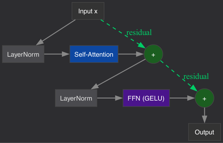
A single transformer block combines attention and feed-forward with residual connections and layer normalization:

class TransformerBlock(nn.Module):
    def __init__(self, config):
        self.ln1 = nn.LayerNorm(embed_dim)
        self.attn = CausalSelfAttention(config)
        self.ln2 = nn.LayerNorm(embed_dim)
        self.ff = FeedForward(config)

    def forward(self, x):
        x = x + self.attn(self.ln1(x))   # attention + residual
        x = x + self.ff(self.ln2(x))     # feedforward + residual
        return x

Residual Connections: Why x + f(x) Instead of Just f(x)?

Without residuals, a 6-layer network means information must pass through 6 transformations in series. Gradients vanish or explode. Training becomes unstable.

With residuals, each layer only needs to learn the delta — what to add to the current representation. If a layer has nothing useful to contribute, it can output near-zero and the input passes through unchanged. This makes deep networks trainable.

Without residuals: x → f₁ → f₂ → f₃ → f₄ (gradients must flow through all)
With residuals:    x → x + f₁(x) → x + f₁(x) + f₂(...) → ... (gradient has direct path)

LayerNorm: Why Normalize?

self.ln1 = nn.LayerNorm(embed_dim)

Training neural networks is sensitive to the scale of activations. If some layers produce values in [0, 1] and others in [-1000, 1000], the learning rate that works for one destroys the other. LayerNorm keeps everything on a consistent scale.

Pre-norm vs post-norm: We use pre-norm (normalize before attention/FF), which is what GPT-2 and most modern models use. The original transformer paper used post-norm. Pre-norm is more stable for training.

Step 5: The Full GPT Model

Stack everything together:

class GPT(nn.Module):
    def __init__(self, config):
        # Embeddings
        self.token_emb = nn.Embedding(config.vocab_size, config.embed_dim)
        self.pos_emb = nn.Embedding(config.context_length, config.embed_dim)
        self.drop = nn.Dropout(config.dropout)

        # N transformer blocks
        self.blocks = nn.Sequential(
            *[TransformerBlock(config) for _ in range(config.n_layers)]
        )

        # Output
        self.ln_final = nn.LayerNorm(config.embed_dim)
        self.head = nn.Linear(config.embed_dim, config.vocab_size, bias=False)

        # Weight tying: output projection shares weights with token embedding
        self.token_emb.weight = self.head.weight

Weight Tying: Why Share Embedding and Output Weights?

The token embedding maps: token ID → vector. The output head maps: vector → token ID probabilities.

These are inverse operations. By sharing the weight matrix, we:

1. Reduce parameter count (no duplicate matrix)
2. Enforce consistency: if two tokens have similar embeddings, they’ll have similar output probabilities
3. Improve training: both the input and output side contribute gradients to the same matrix

Weight Initialization

def _init_weights(self, module):
    if isinstance(module, nn.Linear):
        torch.nn.init.normal_(module.weight, mean=0.0, std=0.02)
        if module.bias is not None:
            torch.nn.init.zeros_(module.bias)
    elif isinstance(module, nn.Embedding):
        torch.nn.init.normal_(module.weight, mean=0.0, std=0.02)

Why std=0.02? At initialization, we want activations to have reasonable magnitude. Too large → exploding gradients. Too small → dead neurons. 0.02 keeps the initial forward pass well-behaved for typical model sizes. GPT-2 used this value.

The Forward Pass — End to End

def forward(self, idx, targets=None):
    B, T = idx.shape

    # 1. Embeddings: token IDs → dense vectors with position info
    pos = torch.arange(0, T, device=idx.device).unsqueeze(0)
    x = self.drop(self.token_emb(idx) + self.pos_emb(pos))

    # 2. Transformer blocks: build contextual representations
    for block in self.blocks:
        x = block(x)

    # 3. Output: project to vocabulary probabilities
    x = self.ln_final(x)
    logits = self.head(x)  # [B, T, vocab_size]

    # 4. Loss (during training): compare predictions to actual next tokens
    loss = None
    if targets is not None:
        loss = F.cross_entropy(
            logits.view(-1, logits.size(-1)),  # flatten to [B*T, vocab_size]
            targets.view(-1),                   # flatten to [B*T]
        )

    return logits, loss

Every position simultaneously predicts its next token. At position 3, the model outputs a probability distribution over all 512 tokens — its best guess for what token 4 should be. During training, we know the answer and compute the loss. During generation, we sample from this distribution.

Our Model’s Configuration

config = Config(
    vocab_size=512,        # number of tokens our BPE tokenizer produces
    context_length=128,    # max sequence length (tokens)
    n_layers=4,            # transformer blocks stacked
    n_heads=4,             # parallel attention heads
    embed_dim=256,         # dimension of all internal representations
    dropout=0.1,           # regularization
)

This gives us 3.3 million parameters. For reference:

• GPT-2 small: 124M parameters
• GPT-3: 175B parameters
• Our model: 3.3M parameters

Same architecture. Different scale. The mechanism is identical.

Parameter Breakdown

Token embedding:      512 × 256 =     131,072  (shared with output head)
Position embedding:   128 × 256 =      32,768
Per transformer block:
  QKV projection:     256 × 768 =     196,608
  Output projection:  256 × 256 =      65,536
  FF layer 1:         256 × 1024 =    262,144
  FF layer 2:         1024 × 256 =    262,144
  LayerNorms (×2):    256 × 2 × 2 =     1,024
  Subtotal per block:                  787,456
× 4 blocks:                          3,149,824
Final LayerNorm:      256 × 2 =            512
─────────────────────────────────────────────
Total:                              ~3,314,000

Most parameters (~95%) are in the transformer blocks. Of those, ~67% are in the feed-forward layers. Attention itself is relatively cheap in parameters — its cost is in compute (the O(n²) matrix multiplication).

---

4. Pretraining

Pretraining has one objective: predict the next token. That’s it. No grammar rules, no world knowledge injected — just next-token prediction via cross-entropy loss. To predict well, the model must learn language structure, facts, and reasoning as side effects.

The Problem

We have a transformer with 3.3 million randomly initialized parameters. Right now, it outputs random noise. We need to find parameter values that make it produce coherent English.

The answer — and this is perhaps the most surprising fact about modern AI — is incredibly simple: predict the next token.

No grammar rules. No world knowledge. No explicit reasoning training. Just: given tokens [0…t], predict token [t+1]. Everything else (grammar, facts, reasoning, creativity) emerges as a side effect of getting good at this one task.

Why Next-Token Prediction Works

This is counterintuitive. How does “autocomplete on steroids” produce intelligence?

The key insight: to predict the next token well, you must understand the text.

Consider predicting the next word in:

“The capital of France is ___”

To get this right, the model must have learned the fact that France’s capital is Paris. It needs world knowledge.

“She picked up the phone and ___”

The model must understand causality, common actions, narrative structure.

“If x² = 4, then x = ___”

The model must have learned mathematical reasoning.

The prediction objective forces the model to build internal representations of grammar, facts, logic, and reasoning — because those representations help it predict better. It’s learning to compress the training data, and compression requires understanding.

Data Format

Training data is simply text, split into chunks of context_length tokens:

class TextDataset:
    def __init__(self, token_ids, context_length):
        self.token_ids = torch.tensor(token_ids, dtype=torch.long)
        self.context_length = context_length

    def __getitem__(self, idx):
        start = idx * self.context_length
        end = start + self.context_length

        x = self.token_ids[start:end]       # input
        y = self.token_ids[start + 1:end + 1]  # target (shifted by 1)
        return x, y

The target is the input shifted by one position:

Input:  [The] [cat] [sat] [on] [the] [mat]
Target: [cat] [sat] [on]  [the] [mat] [.]

Every position simultaneously tries to predict its next token. A single training example of 128 tokens gives us 128 prediction tasks at once.

The Loss Function: Cross-Entropy

loss = F.cross_entropy(
    logits.view(-1, vocab_size),   # model's predictions: [B*T, vocab_size]
    targets.view(-1),               # actual next tokens:  [B*T]
)

Cross-entropy measures: “how surprised was the model by the actual next token?”

• If the model assigns 90% probability to the correct token → loss ≈ 0.1 (good)
• If the model assigns 1% probability to the correct token → loss ≈ 4.6 (bad)
• Random chance (uniform over 512 tokens) → loss ≈ 6.2 (untrained model)

The Training Loop

model.train()
for step in range(max_steps):
    # 1. Get a batch of training data
    x, y = get_batch(train_dataset, batch_size, device)

    # 2. Forward pass: compute predictions and loss
    logits, loss = model(x, y)

    # 3. Backward pass: compute gradients
    loss.backward()

    # 4. Clip gradients (prevent explosion)
    torch.nn.utils.clip_grad_norm_(model.parameters(), 1.0)

    # 5. Update parameters
    optimizer.step()

    # 6. Reset gradients for next step
    optimizer.zero_grad()

The Optimizer: AdamW

optimizer = torch.optim.AdamW(
    model.parameters(),
    lr=3e-4,           # peak learning rate
    weight_decay=0.1,  # L2 regularization
)

Why AdamW and not plain SGD?

SGD (Stochastic Gradient Descent): one learning rate for all parameters. If gradient is 0.001 for one parameter and 1000 for another, one of them gets a terrible update.

Adam (Adaptive Moment Estimation): maintains a per-parameter learning rate. Tracks both the gradient mean (momentum) and gradient variance. Parameters with consistently large gradients get smaller updates; parameters with small, noisy gradients get larger updates.

AdamW = Adam + decoupled weight decay. Weight decay (multiplying all weights by 0.999 each step) is a form of regularization that prevents weights from growing too large. AdamW implements this correctly (plain Adam’s weight decay interacts poorly with the adaptive learning rate).

Every modern LLM uses AdamW.

Learning Rate Schedule: Warmup + Cosine Decay

def get_lr(step):
    # Phase 1: Linear warmup (first 100 steps)
    if step < warmup_steps:
        return (step + 1) / warmup_steps

    # Phase 2: Cosine decay to zero
    progress = (step - warmup_steps) / (max_steps - warmup_steps)
    return 0.5 * (1 + math.cos(math.pi * progress))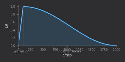

Why warmup? At initialization, the model’s representations are random. Large learning rates push parameters far based on meaningless gradients. Warmup lets the model “settle” into a reasonable region before applying full learning rate.

Why cosine decay? As training progresses, the model is closer to optimal. Smaller updates prevent overshooting. Cosine gives a smooth decay that doesn’t drop too fast (like exponential) or stay too high (like constant).

Gradient Clipping

grad_norm = torch.nn.utils.clip_grad_norm_(model.parameters(), max_norm=1.0)

Occasionally, a batch produces unusually large gradients (a “gradient spike”). Without clipping, one bad batch can destroy hours of training progress by sending parameters to extreme values.

Gradient clipping scales the entire gradient vector so its norm never exceeds 1.0. It preserves the gradient direction but limits its magnitude.

Gradient Accumulation

for micro_step in range(grad_accum_steps):
    x, y = get_batch(train_dataset, batch_size, device)
    logits, loss = model(x, y)
    loss = loss / grad_accum_steps  # normalize
    loss.backward()                 # accumulate gradients

# Only update after all micro-steps
optimizer.step()
optimizer.zero_grad()

The problem: we want a large effective batch size (more stable gradients), but our GPU/memory can only fit a small batch.

The solution: accumulate gradients over multiple forward passes, then do one update. With batch_size=16 and grad_accum_steps=4, the effective batch size is 64 — but we never hold more than 16 samples in memory.

This is how people train large models on limited hardware.

Training Progress

step     0 | train loss 6.2926 | val loss 6.3042  ← random (correct for 512 vocab)
step   100 | train loss 4.7071 | val loss 4.7251  ← learning fast
step   200 | train loss 4.2015 | val loss 4.1096  ← still improving
step   300 | train loss 4.0547 | val loss 3.9854  ← diminishing returns
step   400 | train loss 4.0264 | val loss 3.9230  ← converging

The starting loss (6.29) is close to ln(512) = 6.24 — the theoretical loss for uniform random predictions over 512 tokens. This confirms our model is correctly initialized.

We hold out 10% of the data for validation:

• If training loss drops but validation loss doesn’t → the model is memorizing, not learning
• If both drop together → the model is learning genuine patterns

Running on Apple Silicon (MPS)

def get_device():
    if torch.backends.mps.is_available():
        return torch.device("mps")
    elif torch.cuda.is_available():
        return torch.device("cuda")
    return torch.device("cpu")

Apple’s Metal Performance Shaders backend gives ~4× speedup over CPU. The entire training (2000 steps) completes in ~1 minute on an M-series Mac.

What the Model Learns

After 2000 steps, the loss drops from 6.3 to ~3.4:

• Loss 6.3 → random noise, no English structure
• Loss 5.0 → learns common character patterns (th, er, ing)
• Loss 4.0 → produces word-like sequences, some real words
• Loss 3.5 → mostly recognizable English, some grammar
• Loss 3.0 → (would need more data/parameters) coherent sentences

Output at loss 3.4:

Input: "The "
Output: "The quengerigned and profection, Tweenerved by the mary off"

Not coherent — but recognizably English. Real words mixed with plausible-looking fake ones. With more data and more parameters, this becomes fluent text.

Key Takeaways

1. The objective is absurdly simple. Predict the next token. Understanding emerges from prediction.
2. Stability tricks matter. Without warmup, gradient clipping, and proper initialization, training fails silently.
3. Scale is the secret. Our 3.3M model learns basic patterns. GPT-3’s 175B model learns essays, code, and poetry. Same algorithm, 50,000× more parameters.
4. Compute is accessible. You can pretrain a working language model in 1 minute on a laptop.

---

5. Fine-tuning

Fine-tuning doesn’t teach new knowledge — it teaches new behavior. Same model, same loss function, different data format. By training on instruction-response pairs instead of raw text, the model learns to answer questions instead of continuing them.

The Problem

After pretraining, our GPT can produce English text. But it doesn’t know what you want it to do. Ask it a question, and it might continue with more questions. Give it an instruction, and it might write an article about instructions.

The model has learned language. It hasn’t learned behavior.

Prompt: "What is the capital of France?"

Pretrained model output:
"What is the capital of France? What is the capital of Germany?
What is the capital of Spain?..."
(It learned that questions often come in lists)

Fine-tuned model output:
"The capital of France is Paris."
(It learned that questions should be answered)

What Fine-tuning Actually Does

Fine-tuning does NOT teach the model new knowledge. The knowledge comes from pretraining (it saw “Paris” thousands of times).

Fine-tuning teaches the model a new format: when you see a question/instruction, produce an answer/response. It’s behavioral alignment, not knowledge injection.

The mechanism is identical to pretraining:

• Same loss function (cross-entropy, next-token prediction)
• Same optimizer (AdamW)
• Same forward pass

The only difference is the data format.

The Data Format

Pretraining data (unstructured text):

The cat sat on the mat. It was a warm sunny day and
the birds were singing in the trees outside...

Fine-tuning data (structured instruction-response pairs):

### Instruction:
What is gravity?

### Response:
Gravity is the force that attracts objects with mass toward each other.

The model learns: when I encounter the pattern ### Instruction:\n...\n### Response:\n, what follows should be a direct answer. The special markers act as format tokens that signal the expected behavior.

This is why ChatGPT responds to questions instead of continuing them — it was fine-tuned on millions of (question, answer) pairs.

The Critical Detail: Masking Padding

Instruction-response samples vary in length:

Sample 1: "What is 2+2?" → "4."                    (12 tokens)
Sample 2: "Explain photosynthesis." → "Plants..."    (85 tokens)

The model needs fixed-length sequences for batched training. We pad short sequences. But if we compute loss on padding tokens, the model wastes capacity learning to predict zeros.

The solution: mask the loss on padding positions:

PAD_TOKEN = -100  # PyTorch's special ignore value

def __getitem__(self, idx):
    tokens, seq_len = self.samples[idx]
    x = tokens[:-1]
    y = tokens[1:].clone()

    # Tell cross-entropy to IGNORE these positions
    y[seq_len - 1:] = PAD_TOKEN
    return x, y

loss = F.cross_entropy(
    logits.view(-1, logits.size(-1)),
    targets.view(-1),
    ignore_index=-100,  # ← skip positions where target is -100
)

This seems like a minor detail, but getting it wrong is a common bug that silently degrades model quality.

Differences from Pretraining

Aspect	Pretraining	Fine-tuning
Data	Raw text (5.7MB)	Instruction pairs (20 samples)
Learning rate	3e-4	1e-4 (3× lower)
Weight decay	0.1	0.01 (10× lower)
Steps	2000	500
Purpose	Learn language	Learn behavior

Lower learning rate: the model already has good representations. Large updates would destroy that knowledge. We want small, precise adjustments.

Lower weight decay: we don’t want to regularize away what pretraining learned — we want to preserve it while adding new behavior on top.

Fewer steps: with only 20 training samples, overfitting happens fast. After 500 steps, the model has seen each sample ~100 times.

The Fine-tuning Loop

model.train()
for step in range(max_steps):
    x, y = get_batch(train_dataset, batch_size, device)

    # Forward pass
    logits, _ = model(x)

    # Loss only on non-padded positions
    loss = F.cross_entropy(
        logits.view(-1, logits.size(-1)),
        y.view(-1),
        ignore_index=-100,
    )

    # Standard backward pass
    loss.backward()
    torch.nn.utils.clip_grad_norm_(model.parameters(), 1.0)
    optimizer.step()
    optimizer.zero_grad()

Structurally identical to pretraining. The model doesn’t “know” it’s being fine-tuned.

What Changes in the Model

Fine-tuning modifies ALL parameters. But the changes are small:

Pretrained weights:  W = [learned language structure]
Fine-tuned weights:  W' = W + δ  (small perturbation)

The model retains its language ability and gains instruction-following behavior.

Advanced: LoRA (Low-Rank Adaptation)

For larger models, fine-tuning all parameters is expensive. LoRA freezes the original weights and trains small “adapter” matrices:

Original: y = Wx
LoRA:     y = Wx + BAx  (where B and A are small matrices)

W is frozen (175B parameters → no gradients, no optimizer state)
B×A is trained (maybe 1M parameters → cheap)

We don’t use LoRA in our tiny model (3.3M params is already cheap to fine-tune fully). But it’s how GPT-4, Claude, and other production models are adapted.

Results

Before fine-tuning:

Prompt: "### Instruction:\nWhat is gravity?\n\n### Response:\n"
Output: "...and the bright stars which would of a little of the creature..."

After fine-tuning:

Prompt: "### Instruction:\nWhat is gravity?\n\n### Response:\n"
Output: "Gravity is the force that attr..." (truncated)

The quality is limited by our model’s tiny size — 3.3M parameters can’t store much factual knowledge. But the format is correct: it generates a response instead of continuing randomly. The mechanism works.

The Full Pipeline So Far

Raw text                     → BPE Tokenizer    → Token IDs
Token IDs + Random Weights   → Pretraining      → Language Model
Language Model + Instruction Data → Fine-tuning  → Instruction-Following Model

Three stages, each building on the last. The architecture never changes:

1. Tokenizer: learn compression
2. Pretraining: learn language
3. Fine-tuning: learn behavior

Key Takeaways

1. Fine-tuning is format training, not knowledge training. The model already “knows” facts from pretraining. Fine-tuning teaches it when and how to express them.
2. The loss function is identical. No special “alignment loss.” The structure of the data does all the work.
3. Mask your padding. If you don’t ignore padded positions in the loss, the model learns to generate padding — a subtle but impactful bug.
4. Less is more. Lower learning rate, lower regularization, fewer steps. It’s a delicate adjustment, not a heavy training run.
5. This is how ChatGPT was made. Pretrain on the internet (expensive, done once) → fine-tune on conversations (cheap, done repeatedly).

---

6. Inference

Naive generation recomputes all previous tokens every step — O(n²) total. KV cache stores past Keys and Values so each new token only computes one query against the cached context — O(n) total. This is how every production LLM serves responses fast.

The Problem

The model is trained. Now we need to generate text. Two critical challenges:

1. Speed: the naive approach is O(n²) per generated token. For long sequences, unacceptably slow.
2. Quality: the model outputs probabilities, not words. How you convert probabilities to tokens dramatically affects output quality.

How Autoregressive Generation Works

GPT generates text one token at a time:

Step 1: Input "The"       → Model predicts next token → "cat"
Step 2: Input "The cat"   → Model predicts next token → "sat"
Step 3: Input "The cat sat" → Model predicts next token → "on"
...

Naive code (no optimization):

for i in range(max_new_tokens):
    # Feed ENTIRE sequence every time
    x_cond = x[:, -context_length:]  # truncate if too long
    logits, _ = model(x_cond)        # full forward pass
    logits = logits[:, -1, :]        # only the last position matters
    next_token = sample(logits)      # pick a token
    x = torch.cat([x, next_token], dim=1)  # append

The problem: at step 100, we process 100 tokens through all layers. At step 200, we process 200 tokens. Most of this computation is redundant.

The KV Cache: The Key Optimization

The Insight

In causal self-attention: past tokens’ Keys and Values never change.

When generating token 50, the Key and Value vectors for tokens 0–49 are identical to what they were when we generated token 49. The causal mask guarantees this.

So why recompute them?

How It Works

Quadratic → linear. For generating 100 tokens with context 100, that’s ~100× less compute.

The Two Phases

Phase 1 — Prefill: Process the entire prompt at once. This populates the cache.

model.clear_cache()
logits, _ = model(prompt_tokens, use_cache=True, pos_offset=0)
# Cache now holds K,V for all prompt tokens

Phase 2 — Decode: Generate tokens one at a time, using the cache.

for i in range(max_new_tokens):
    pos_offset = current_sequence_length - 1
    logits, _ = model(last_token_only, use_cache=True, pos_offset=pos_offset)
    next_token = sample(logits)

Implementation in the Attention Layer

class CausalSelfAttention(nn.Module):
    def __init__(self, config):
        ...
        self.cache_k = None
        self.cache_v = None

    def clear_cache(self):
        self.cache_k = None
        self.cache_v = None

    def forward(self, x, use_cache=False):
        B, T, C = x.shape

        # Compute Q, K, V for the NEW tokens only
        qkv = self.qkv(x)
        q, k, v = qkv.split(C, dim=-1)
        # reshape to [B, n_heads, T, head_dim]...

        if use_cache:
            if self.cache_k is not None:
                # Append new K,V to cached K,V
                k = torch.cat([self.cache_k, k], dim=2)
                v = torch.cat([self.cache_v, v], dim=2)
            # Update cache
            self.cache_k = k
            self.cache_v = v

        # Attention: new Q attends to ALL K (cached + new)
        # q: [B, heads, T_new, head_dim]  (usually T_new = 1 during decode)
        # k: [B, heads, T_total, head_dim] (all cached + new)
        attn = (q @ k.transpose(-2, -1)) * (head_dim ** -0.5)
        ...

During decode, T_new = 1 (one new token) and T_total grows by 1 each step. The attention computation is just one query attending to N keys — a vector-matrix multiply instead of a matrix-matrix multiply.

Position Encoding with Cache

def forward(self, idx, use_cache=False, pos_offset=0):
    B, T = idx.shape

    # Position is NOT always 0,1,2,...T
    # During decode, it's the absolute position: e.g., 57 for the 58th token
    pos = torch.arange(pos_offset, pos_offset + T, device=idx.device)
    x = self.token_emb(idx) + self.pos_emb(pos)

Without pos_offset, every decode step would use position embedding 0 — the model would think every token is the first token. This is a subtle but critical bug.

When Cache Doesn’t Help

KV cache adds overhead (memory for stored tensors, torch.cat operations). For our tiny model (3.3M params, context_length=128), the overhead exceeds the savings. The cache starts paying off with:

• Larger models (more computation per layer)
• Longer sequences (more redundant recomputation to avoid)
• Production serving (where latency matters)

At GPT-4 scale, KV cache isn’t optional — it’s the difference between 2 seconds and 2 minutes per response.

Sampling: Turning Probabilities into Text

The model outputs logits: one number per vocabulary token. Higher logit = more likely token. But we need to pick ONE token.

Greedy Decoding (Always Pick the Most Likely)

next_token = logits.argmax(dim=-1)

Pros: deterministic, “safest” choice. Cons: repetitive, boring, often loops (“the the the the…”).

Why it loops: if “the” is the most likely token in some context, greedy always picks it, creating a context where “the” is again most likely. Almost never used for open-ended generation.

Temperature: Controlling Randomness

logits = logits / temperature
probs = softmax(logits)
next_token = multinomial(probs, num_samples=1)

Temperature reshapes the probability distribution:

Original logits: [2.0, 1.0, 0.5, -1.0]
Softmax:         [0.47, 0.17, 0.10, 0.02]  (roughly)

Temperature = 0.5 (sharper):
Scaled logits:   [4.0, 2.0, 1.0, -2.0]
Softmax:         [0.84, 0.11, 0.04, 0.00]  ← top token dominates

Temperature = 2.0 (flatter):
Scaled logits:   [1.0, 0.5, 0.25, -0.5]
Softmax:         [0.34, 0.21, 0.16, 0.08]  ← more uniform

• Low temperature (0.2–0.5): very confident, coherent but repetitive
• Temperature = 1.0: model’s original distribution, natural variety
• High temperature (1.5–2.0): all tokens more likely, creative but potentially incoherent

Top-k Sampling: Limiting Choices

# Only consider the k most probable tokens
top_k_values, _ = torch.topk(logits, k=40)
threshold = top_k_values[:, -1:]
logits[logits < threshold] = float("-inf")  # zero out everything else

probs = softmax(logits)
next_token = multinomial(probs)

The problem: even with reasonable temperature, low-probability tokens sometimes get sampled. Token 500 with 0.001% probability is almost certainly wrong.

Top-k says: only consider the top 40 candidates. Everything else is impossible.

The limitation: k=40 is fixed. Sometimes the model is very confident (2 tokens have 90% combined probability) and sometimes uncertain (100 tokens each have 1%). A fixed k doesn’t adapt.

Top-p (Nucleus) Sampling: Adaptive Filtering

sorted_logits, sorted_idx = torch.sort(logits, descending=True)
cumulative_probs = torch.cumsum(softmax(sorted_logits), dim=-1)

# Keep tokens until cumulative probability exceeds p
mask = cumulative_probs - softmax(sorted_logits) >= top_p
sorted_logits[mask] = float("-inf")

Top-p keeps the smallest set of tokens whose combined probability exceeds p (e.g., 0.9).

• If the model is confident: “Paris” has 85% → only 2-3 tokens in the nucleus
• If the model is uncertain: many tokens at 2-3% each → 30-40 tokens in the nucleus

This adapts to the model’s confidence.

Combining Them

In practice, we use all three together:

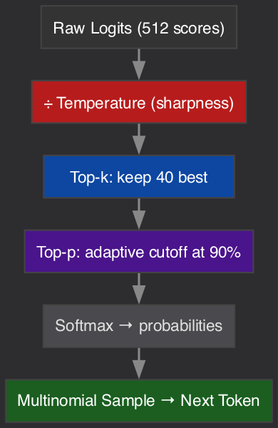
logits = logits / temperature     # reshape distribution
logits = top_k_filter(logits, k)  # remove long tail
logits = top_p_filter(logits, p)  # adaptive narrowing
probs = softmax(logits)
next_token = multinomial(probs)

Good defaults: temperature=0.8, top_k=40, top_p=0.9

The Full Generation Function

def generate(model, tokenizer, prompt, max_new_tokens=200,
             temperature=0.8, top_k=40, top_p=0.9, use_cache=True):
    model.eval()
    token_ids = tokenizer.encode(prompt)
    x = torch.tensor([token_ids], device=device)

    with torch.no_grad():  # no gradients needed for inference
        if use_cache:
            model.clear_cache()

            # PREFILL: process prompt, populate cache
            logits, _ = model(x, use_cache=True, pos_offset=0)
            logits = logits[:, -1, :] / temperature
            next_token = sample(logits, top_k, top_p)
            x = torch.cat([x, next_token], dim=1)

            # DECODE: one token at a time using cache
            for i in range(1, max_new_tokens):
                pos_offset = x.shape[1] - 1
                if pos_offset >= model.config.context_length:
                    break  # can't exceed context window
                logits, _ = model(x[:, -1:], use_cache=True, pos_offset=pos_offset)
                logits = logits[:, -1, :] / temperature
                next_token = sample(logits, top_k, top_p)
                x = torch.cat([x, next_token], dim=1)

            model.clear_cache()

    return tokenizer.decode(x[0].tolist())

Key details:

• model.eval(): disables dropout (deterministic behavior during inference)
• torch.no_grad(): disables gradient tracking (saves memory)
• pos_offset: ensures correct positional encoding for cached generation
• Context length check: stops if we hit the model’s maximum sequence length

Performance Considerations

Memory

KV cache memory per layer = 2 × batch_size × n_heads × seq_len × head_dim × sizeof(float)

For our model: 2 × 1 × 4 × 128 × 64 × 4 bytes = 262 KB per layer × 4 layers = ~1MB

For GPT-4 scale (128 layers, 96 heads, 8K context, 128 head_dim): ~384GB

This is why serving large models is expensive — the KV cache alone can exceed GPU memory.

Latency

Two metrics matter:

• Time to First Token (TTFT): how long the prefill takes (proportional to prompt length)
• Time per Output Token (TPOT): how fast decode generates (one forward pass of 1 token)

For our model on MacBook MPS:

• Prefill: ~5ms for 128 tokens
• Decode: ~15ms per token (~65 tokens/second)

Running the Full Pipeline

# Complete pipeline: download → tokenize → train → finetune → generate
python run.py

# Or just interactive generation with existing checkpoint
python generate.py

Interactive mode:

>>> The meaning of life is
The meaning of life is the great force of those
considerations which the character, and the more
profoundly interested in the subject...

>>> ### Instruction:\nExplain gravity.\n\n### Response:\n
Gravity is the force that attracts objects...

Key Takeaways

1. KV cache is the fundamental inference optimization. O(n²) → O(n). Every production LLM uses it.
2. Prefill and decode are different computational profiles. Prefill is compute-bound (many tokens in parallel). Decode is memory-bound (reading cached KV for one new token).
3. Sampling strategy controls the creativity/coherence tradeoff. Temperature, top-k, and top-p work together. No single “right” setting.
4. The model has a fixed context window. It cannot process or generate beyond context_length tokens.
5. Generation is embarrassingly simple. Predict next token, append, repeat. All the complexity is in the trained model.

---

The Complete Picture

We’ve built a complete GPT from scratch:

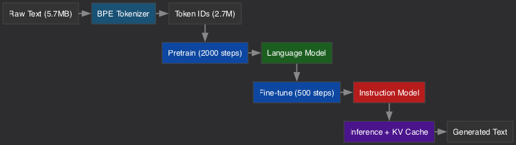
download_data.py  → Get text corpus
tokenizer.py      → BPE tokenization (text → numbers)
model.py          → Transformer architecture
train.py          → Pretraining (learn language)
finetune.py       → Fine-tuning (learn behavior)
generate.py       → Inference (produce text with KV cache)

~500 lines of Python. Same architecture as GPT-4. Running on a MacBook.

The gap between our 3.3M model and GPT-4’s ~1.8T parameters is scale, not mechanism. More layers, more heads, more data, more compute — but the same attention, the same next-token prediction, the same sampling loop.

Full code: github.com/the-last-programmers/gpt-from-scratch