Visualizing Every Step of LLM Inference — Inside a 64M Parameter Model

TL;DR

We load a real 64M-parameter language model (MiniMind-3), ask it “What is AI?”, and trace every computation from raw text to generated response — with actual numbers, actual weight matrices, and actual probability distributions. No abstractions, no black boxes.

---

Why This Article Exists

Most explanations of LLM inference describe it abstractly: “the model predicts the next token.” But what does that actually mean? What are the numbers? What shape are the matrices? What does the attention pattern really look like?

This article answers those questions with a concrete example. We use a real trained model — small enough to inspect every tensor, but architecturally identical to GPT, LLaMA, and Qwen. Every visualization in this article is generated from actual model weights and actual inference computations, not from toy illustrations.

The model: MiniMind-3 — a 64M-parameter decoder-only transformer with 8 layers, 8 attention heads, GQA (4 KV heads), SwiGLU MLP, RoPE, and RMSNorm. It’s architecturally aligned with Qwen3, just 2,700× smaller than GPT-3.

The prompt: "What is AI?"

The goal: See every matrix multiply, every attention score, every probability — from input text to output token.

---

The Complete Inference Pipeline

Before diving into details, here’s the full map. Every section below corresponds to one box:

"What is AI?"
     │
     ▼
┌─────────────────────┐
│  Step 1: Tokenize   │  Text → 21 integer IDs
└─────────┬───────────┘
          ▼
┌─────────────────────┐
│  Step 2: Embed      │  21 IDs → 21 vectors of 768 dims (row lookup)
└─────────┬───────────┘
          ▼
┌─────────────────────┐
│  Step 3: Transform  │  8 layers × (Attention + MLP)
│  (×8 layers)        │  Tokens communicate and "think"
└─────────┬───────────┘
          ▼
┌─────────────────────┐
│  Step 4: LM Head    │  768-dim vector → 6,400 scores
└─────────┬───────────┘
          ▼
┌─────────────────────┐
│  Step 5: Sample     │  6,400 scores → 1 token (temperature, top-p)
└─────────┬───────────┘
          ▼
     "AI" ← Append to input, repeat from Step 2

---

Step 1: Tokenization — Text Becomes Numbers

A language model cannot process text directly. It works with integers — token IDs from a fixed vocabulary. The tokenizer splits text into subword pieces and maps each to a unique ID.

But before tokenization, the raw prompt gets wrapped in a chat template — special tokens that tell the model the conversation structure:

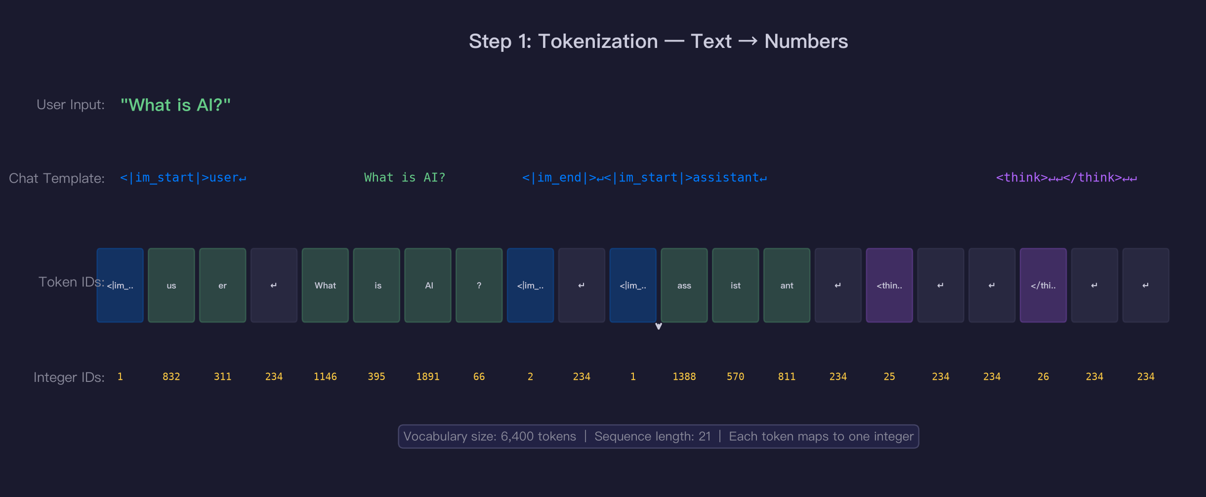
Several things to notice:

1. The vocabulary is small: only 6,400 tokens (compare: LLaMA-3 uses 128K, GPT-4 uses ~100K). This means common words like “What” are single tokens, but rare words get split into subword pieces.

2. Special tokens carry structure: <|im_start|> and <|im_end|> mark message boundaries. <think> and </think> are chain-of-thought reasoning tags — the chat template always includes them, and the model can fill in reasoning between them when needed (empty here).

3. “user” becomes two tokens: us (ID 832) + er (ID 311). The tokenizer learned these as separate subwords.

4. The output is just a list of integers: [1, 832, 311, 234, 1146, 395, 1891, 66, 2, ...]

Property	Value
Input text	“What is AI?”
After chat template	21 tokens
Vocabulary size	6,400
Representation	int32 tensor, shape [1, 21]

Cost: Tokenization is essentially a dictionary lookup — negligible compute compared to what follows.

---

Step 2: Embedding — Row Lookup from a Giant Dictionary

Each token ID is used as an index into the embedding table — a matrix of shape [6400, 768]. Row 1146 is the vector for “What”, row 1891 is the vector for “AI”, and so on.

This is not a computation — it’s a table lookup. The model simply copies 21 rows (one per token) from the 6,400-row table:

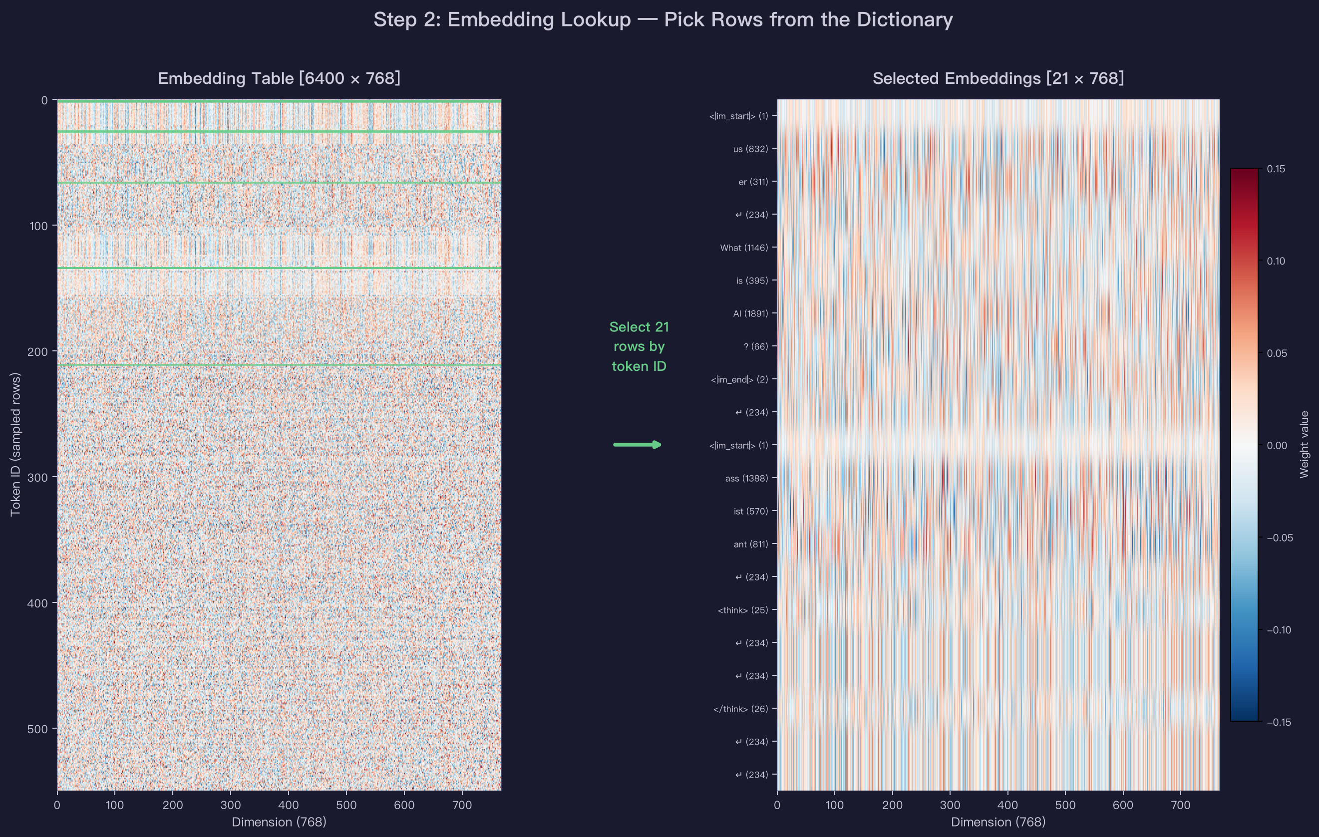
Left: The full embedding table — 6,400 rows × 768 columns. Each row is one token’s “meaning vector” — 768 learned numbers that represent what that token means in a high-dimensional space.

Right: The 21 rows selected by our input token IDs. This is the input to the transformer.

Each of these 768-dimensional vectors was learned during training. The model adjusted these numbers millions of times so that semantically similar words end up with similar vectors:

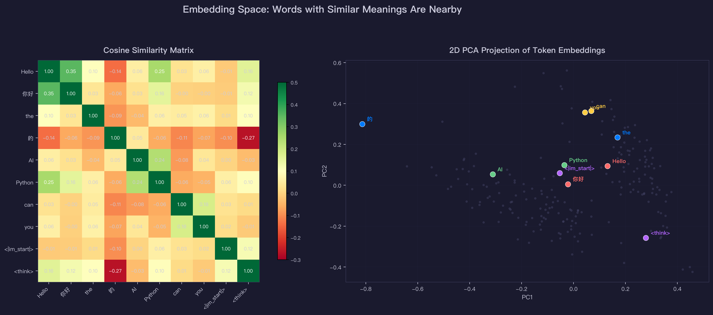
Notice: “Hello” and “你好” (the Chinese greeting) have a cosine similarity of 0.35 — the model learned they’re related despite being in different languages. “AI” and “Python” are also nearby (0.24) — both tech terms. Special tokens like <|im_start|> sit far from regular words.

Property	Value
Embedding table shape	[6400, 768]
Parameters	4.9M (7.7% of the model)
Output shape	[1, 21, 768] — 21 tokens, each a 768-dim vector
Operation	Pure index lookup, no matrix multiplication

---

Step 3: The Transformer Layers — Where Everything Happens

The 21 embedding vectors now pass through 8 identical transformer layers (each with different learned weights). Every layer has the same structure:

Input [21 × 768]
  ├── RMSNorm → Self-Attention → + Residual
  └── RMSNorm → Feed-Forward (SwiGLU) → + Residual
Output [21 × 768]

Let’s walk through each component with real data.

3a: RMSNorm — Stabilizing Values

Before each sub-layer, values are normalized using RMSNorm. This prevents numbers from growing too large or too small across layers:

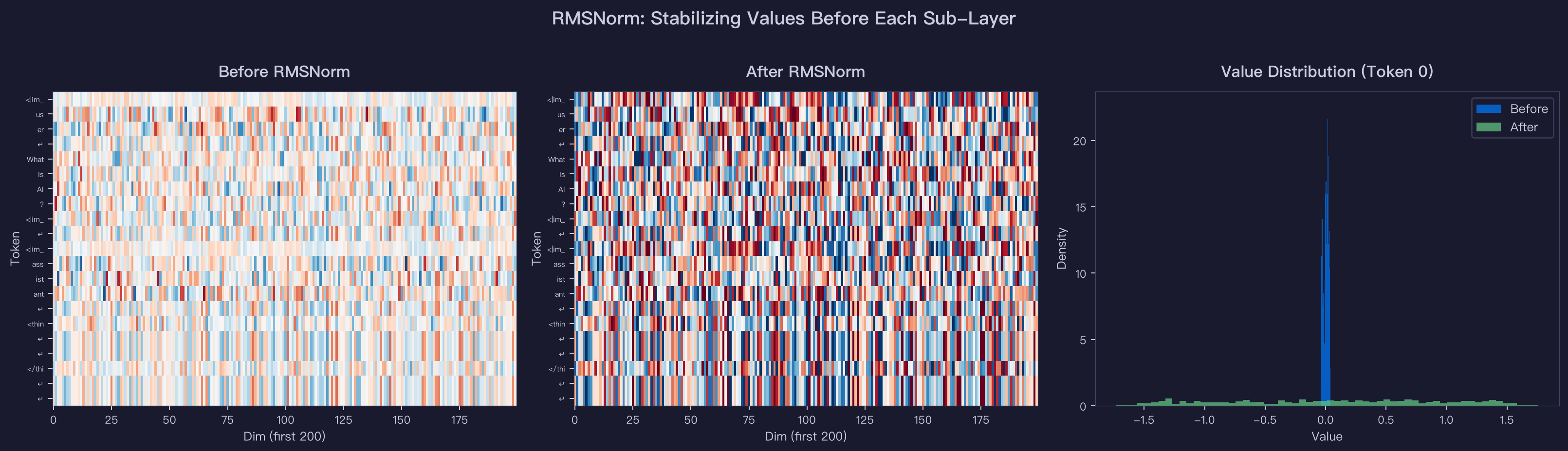
Before normalization: values are tiny (±0.05), clustered near zero. After: values span a wider, more uniform range (±1.5). The histogram shows how the distribution transforms — from a tight spike to a healthy spread.

RMSNorm has only 768 learnable parameters (a per-dimension scale factor) — trivial compared to the attention and MLP weights.

$$\text{RMSNorm}(x) = \frac{x}{\sqrt{\frac{1}{d}\sum_{i=1}^{d} x_i^2 + \epsilon}} \cdot \gamma$$

3b: Self-Attention — Tokens Communicate

This is the mechanism that lets each token “look at” every previous token and gather relevant context. For our 21-token input, attention computes:

1. Q (Query): “What am I looking for?” — shape [21, 8 heads, 96 dims]
2. K (Key): “What do I contain?” — shape [21, 4 heads, 96 dims] (GQA: fewer K heads)
3. V (Value): “What information to pass?” — shape [21, 4 heads, 96 dims]
4. Attention scores = softmax(Q·K^T / √96) — “how much to attend to each other token”
5. Output = scores × V — weighted mix of all tokens’ values

Here are the actual attention patterns from all 8 heads in Layer 0 (early) and Layer 7 (final):

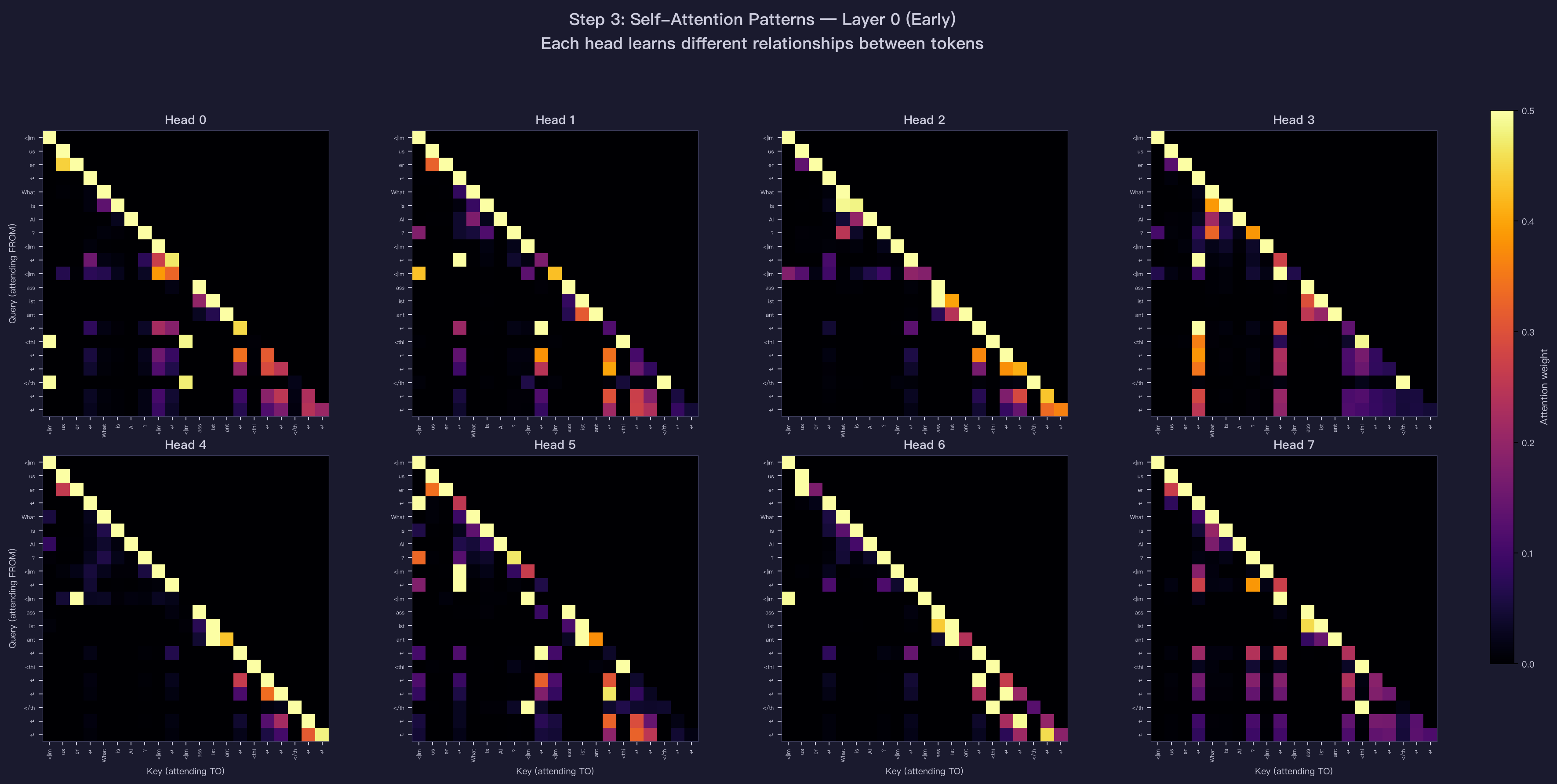
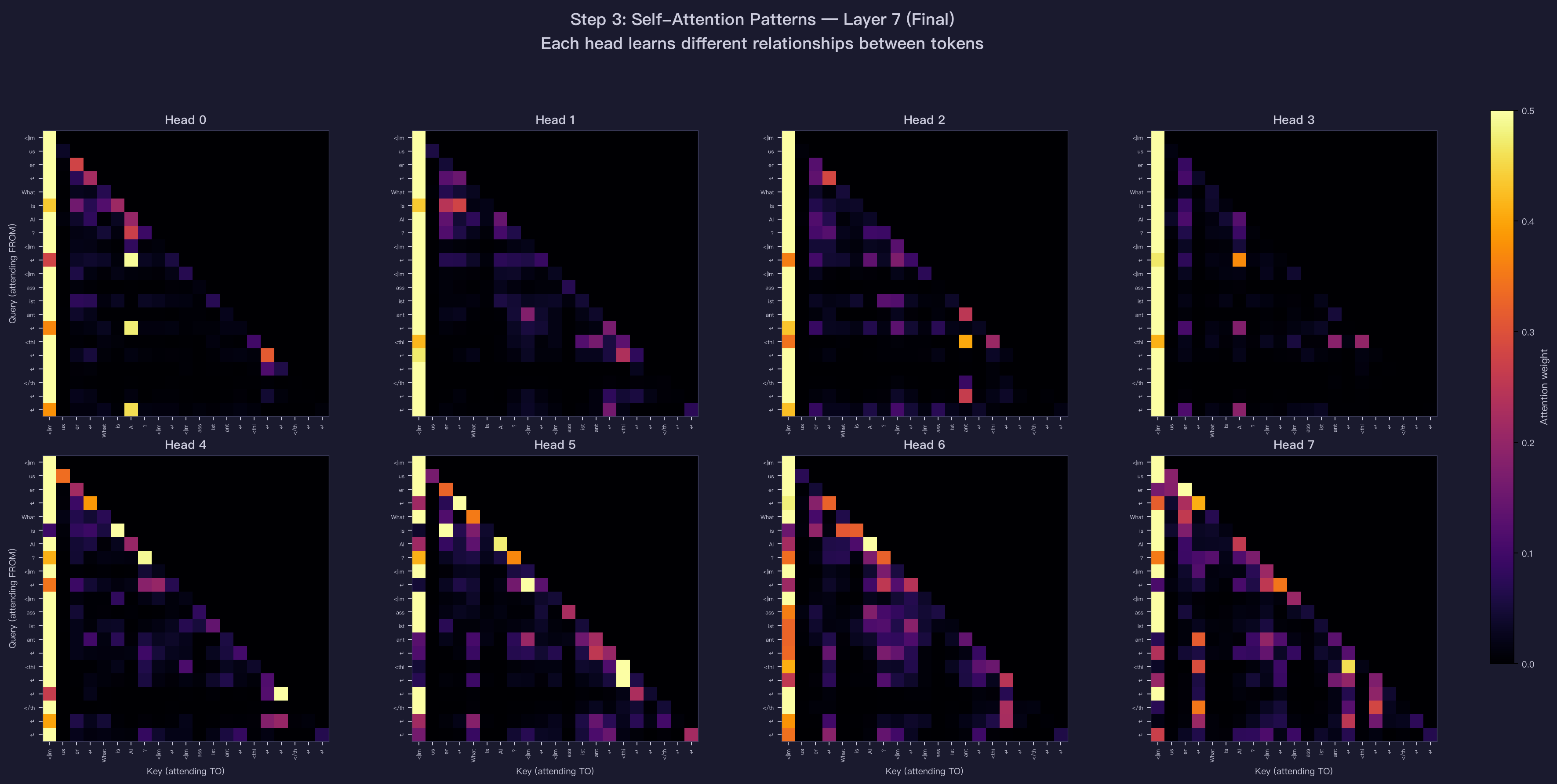
Reading these heatmaps: each row is a query token (“attending FROM”), each column is a key token (“attending TO”). Brighter = higher attention weight. The upper-right triangle is black — that’s the causal mask preventing tokens from attending to future tokens.

Key observations:

• Layer 0 heads are diffuse: attention is spread somewhat evenly — the model is still gathering basic context.
• Layer 7 heads are sharp and specialized: Head 7 shows a strong diagonal pattern (each token attends to the one just before it). Head 2 concentrates on specific content tokens. Head 6 focuses on the special tokens.
• Different heads learn different patterns: Head 3 focuses on the <|im_start|> token across layers. Head 7 is almost purely local attention.

Property	Value
Weight matrices	Q: [768, 768], K: [384, 768], V: [384, 768], O: [768, 768]
Parameters per layer	1.77M (24% of layer, 22% of model)
FLOPs per layer (prefill, 21 tokens)	~75M (projections) + ~1.4M (attention scores)
Attention pattern shape	[8 heads, 21, 21]

3c: Feed-Forward Network (SwiGLU) — Where Knowledge Lives

After attention mixes information between tokens, the MLP processes each token independently. This is where 65% of each layer’s parameters reside — and where most of the model’s factual knowledge is believed to be stored.

The SwiGLU architecture works in three steps:

input [21 × 768]
  ├── gate_proj [768 → 2432] → SiLU activation → gate
  ├── up_proj   [768 → 2432]                    → up
  │   gate × up (element-wise)                   → combined
  └── down_proj [2432 → 768]                     → output

Here’s what the actual tensors look like at each stage:

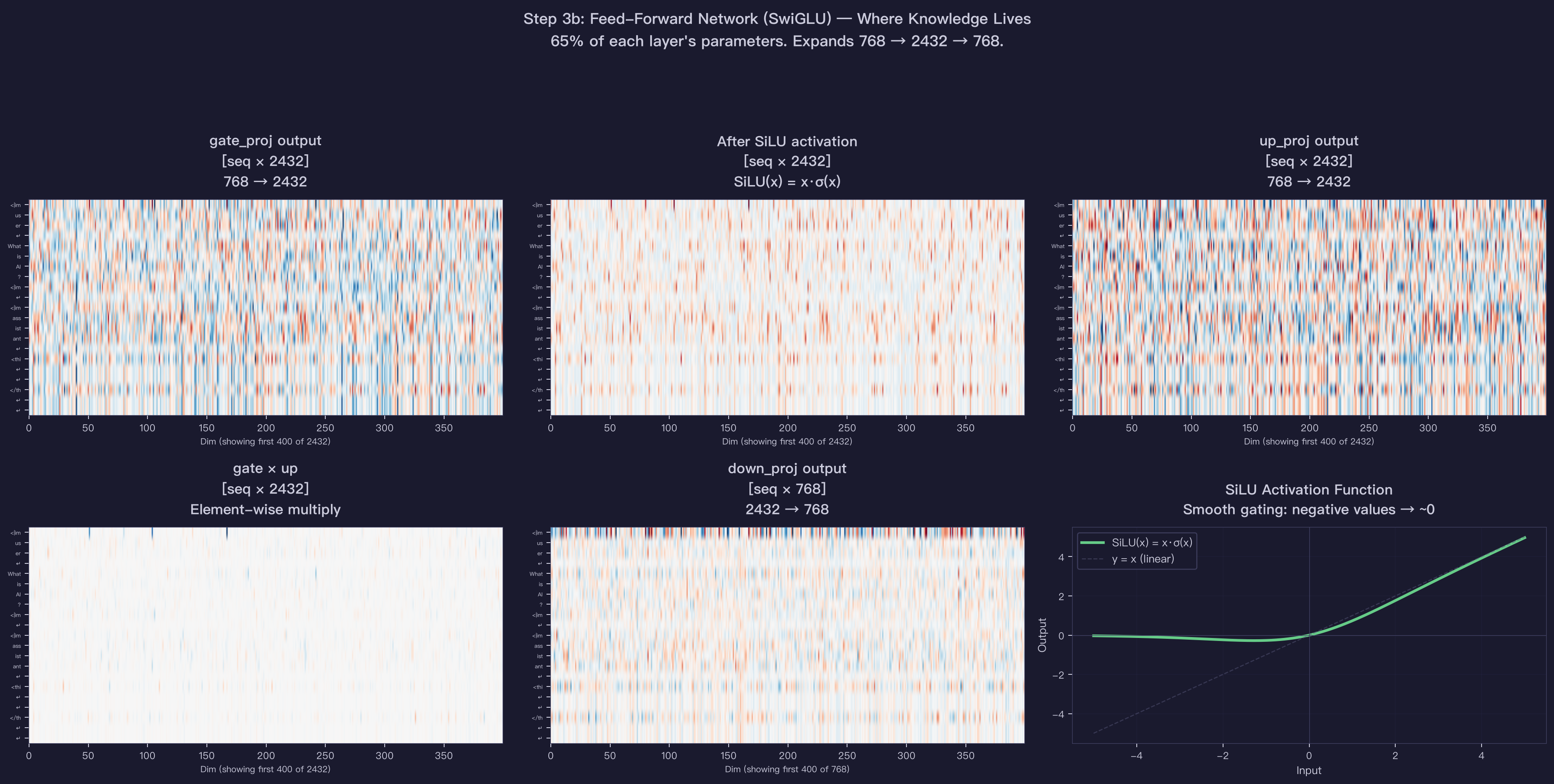
Top-left: The raw gate projection output — expanded from 768 to 2,432 dimensions. Top-middle: After SiLU activation — negative values are suppressed, creating a gating signal. Top-right: The up projection — the “content” pathway. Bottom-left: gate × up — the gate controls which information flows through. Bottom-right: The SiLU function itself — a smooth gate where negative inputs produce near-zero outputs.

The expansion ratio (768 → 2,432 → 768) is where the model’s capacity comes from. The wider intermediate representation allows richer transformations before compressing back.

Property	Value
Weight matrices	gate: [2432, 768], up: [2432, 768], down: [768, 2432]
Parameters per layer	5.6M (76% of layer, 70% of model)
Intermediate dimension	2,432 (≈ 768 × π, rounded to multiple of 64)
Total MLP params (×8 layers)	44.8M

3d: Residual Connections — Adding, Not Replacing

After both attention and MLP, the output is added to the input (not replaced):

output = input + attention(norm(input))
output = output + mlp(norm(output))

This “residual connection” is critical — it lets each layer add a small refinement instead of overwriting everything. Without it, deep networks are nearly impossible to train.

3e: How Hidden States Evolve Across All 8 Layers

Here’s the most revealing visualization — watch how the 21 token representations transform from the raw embedding through all 8 layers:

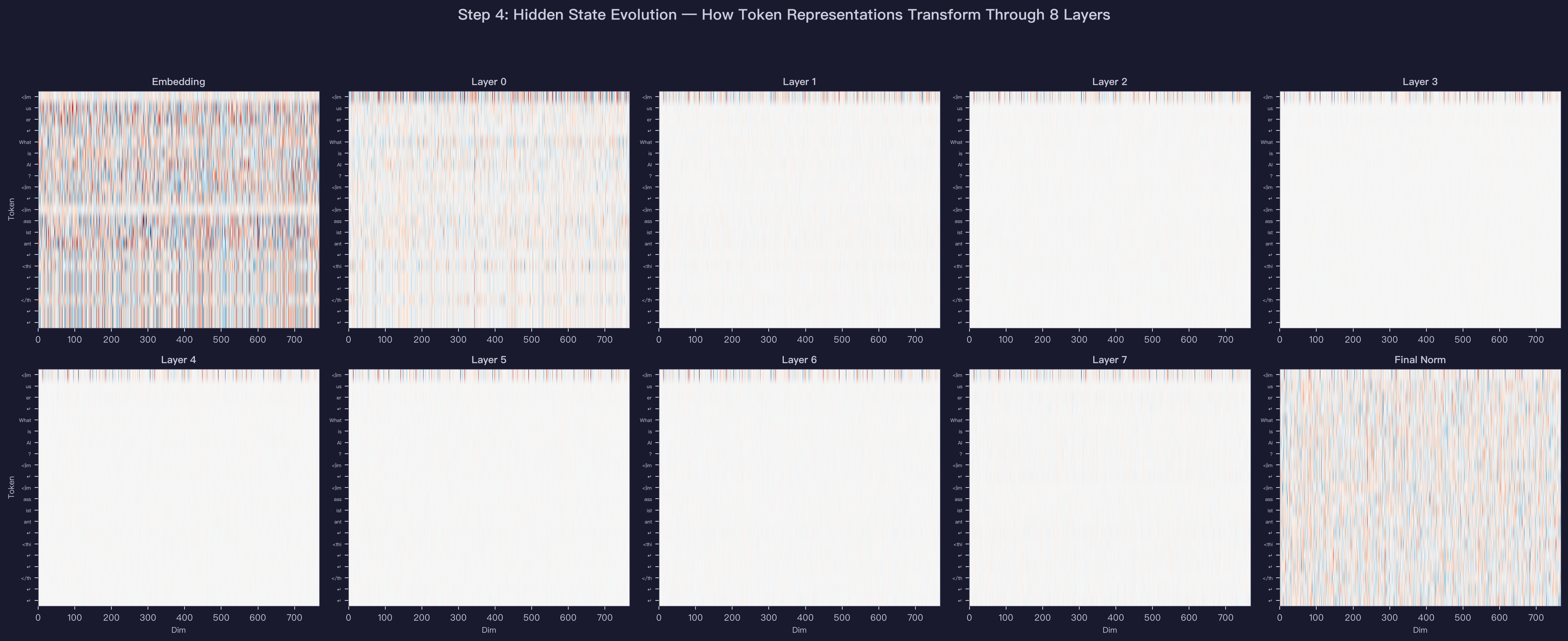
Embedding (far left): All tokens look somewhat similar — they carry only their own meaning. After Layer 7 (near right): Each token has a completely unique, complex pattern — it now carries information about the entire context, not just itself. Final Norm: Values are rescaled one last time before the LM head.

This is the core insight: each layer refines the representation, gradually building up a richer understanding of the full input. The last position’s vector (bottom row) ultimately encodes everything the model needs to predict the next token.

---

Step 4: LM Head — From 768 Dimensions to 6,400 Scores

After 8 transformer layers and a final RMSNorm, we have one 768-dimensional vector per token. We only care about the last position — that’s where the model predicts what comes next.

The LM head multiplies this 768-dim vector by a [6400, 768] weight matrix to produce 6,400 raw scores — one for every word in the vocabulary:

$$\text{logits} = \text{hidden\_state}_{[-1]} \cdot W_{\text{embed}}^T \in \mathbb{R}^{6400}$$

A key design choice: the LM head and the embedding table from Step 2 share the exact same matrix. This is called weight tying. The embedding maps token ID → vector (lookup a row); the LM head reverses this, computing the dot product of the hidden state against every row to find which token it’s closest to.

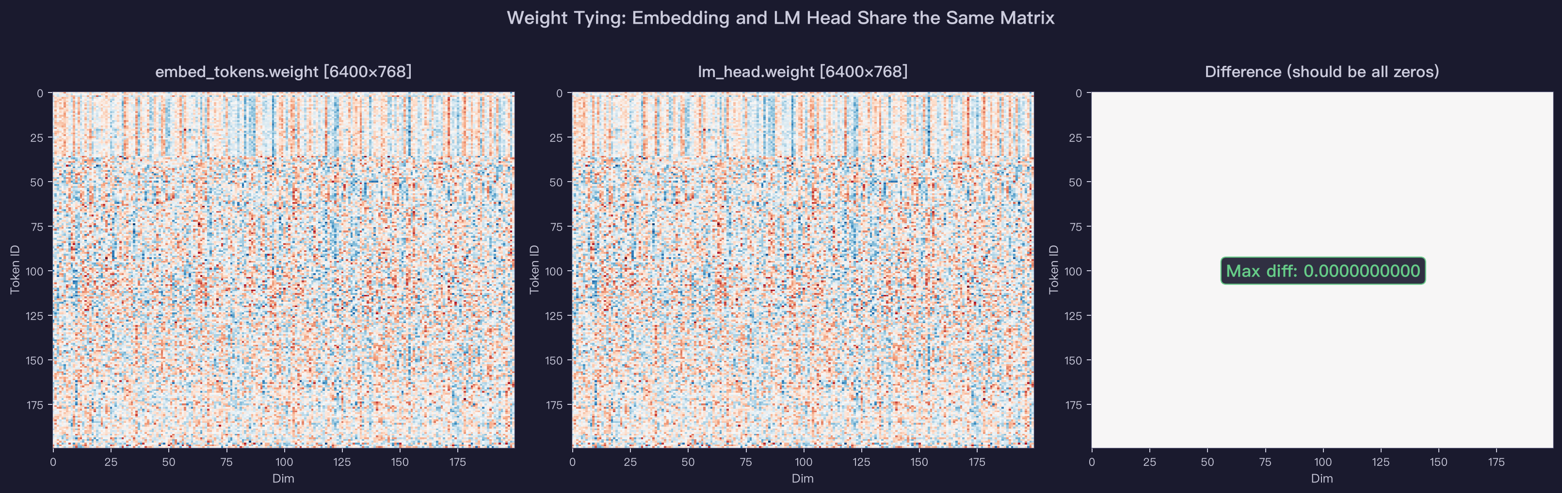
The difference panel (right) is all zeros — confirming these are literally the same tensor in memory, not just similar copies. This saves 4.9M parameters and creates a symmetric relationship: tokens that are “close” in embedding space will also receive high logit scores.

These raw scores are called logits — they’re not yet probabilities.

---

Step 5: Sampling — From 6,400 Scores to 1 Token

This is the final step for each generated token: converting 6,400 raw scores into a single chosen word.

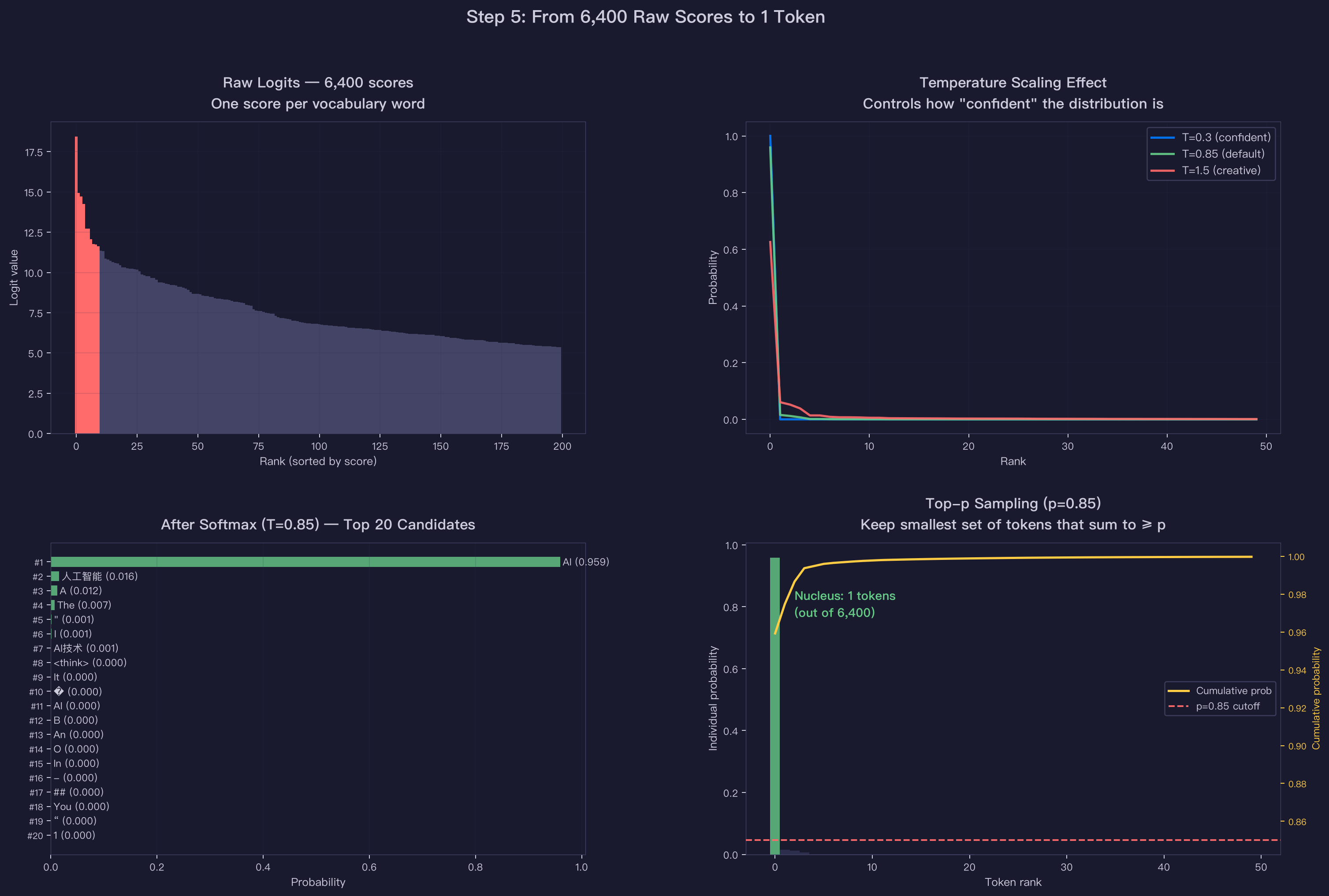
5a: Raw Logits (top-left)

The model outputs 6,400 scores. Most are low (the model is quite sure most words are wrong). A handful have high scores — those are the candidates.

5b: Temperature Scaling (top-right)

Logits are divided by the temperature parameter before softmax:

$$\text{scaled\_logits} = \frac{\text{logits}}{T}$$

• T = 0.3 (blue): Very peaked — the model almost deterministically picks the top token.
• T = 0.85 (green, default): A balance of confidence and creativity.
• T = 1.5 (red): Flat distribution — more random, more “creative” but potentially less coherent.

5c: Softmax Probabilities (bottom-left)

After temperature scaling, softmax converts logits to probabilities that sum to 1.0. For our prompt “What is AI?”, the top candidate is “AI” with 95.9% probability. The runner-up is “人工智能” (Chinese for “artificial intelligence”) at 1.6%.

5d: Top-p (Nucleus) Sampling (bottom-right)

Rather than considering all 6,400 tokens, top-p sampling keeps only the smallest set whose cumulative probability exceeds $p$ (here, 0.85). For this confident prediction, the nucleus is just 1 token — the model is effectively certain.

The green bars are the tokens kept in the nucleus; gray bars are discarded. The yellow line shows the cumulative probability climbing past the 0.85 threshold (red dashed line).

Property	Value
Logits shape	[6400]
Temperature	0.85
Top-p	0.85
Nucleus size (this step)	1 token
Chosen token	“AI” (probability 95.9%)

---

Step 6: The Autoregressive Loop — One Token at a Time

The chosen token (“AI”) is appended to the input, and the entire process repeats from Step 2. The model now has 22 tokens as input and predicts token 23, then 23 → 24, and so on until it generates the EOS (end-of-sequence) token.

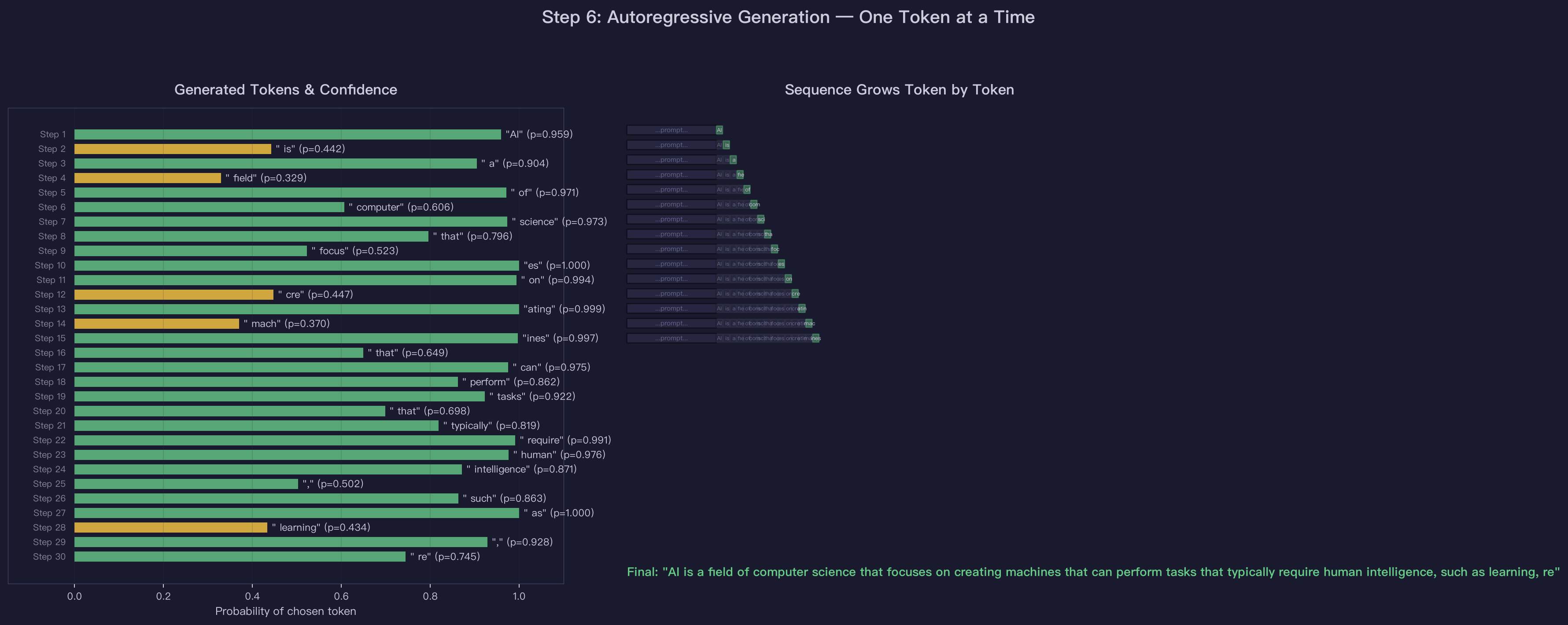
Left panel: Each generated token and its probability. The first token “AI” has 95.9% confidence. Some tokens like “is” and “a” are near-certain (the model knows the grammar). More content-rich words have lower probabilities — the model is “less sure” about which specific word to use.

Right panel: The sequence growing token by token. At each step, the entire history (prompt + all previously generated tokens) is fed through the model to produce the next one.

This is fundamentally sequential — each token depends on all previous ones. In practice, the model doesn’t recompute everything from scratch each step: a KV cache stores the Key and Value tensors from previous positions, so each decode step only processes the single new token against the cached context. But the sequential dependency remains — you can’t generate token $n+1$ without first generating token $n$.

This is why LLM inference is memory-bandwidth-bound during decoding (each step reads all model weights for just one new token) and why techniques like KV caching, speculative decoding, and continuous batching exist.

---

The Full Picture: Compute & Memory

Where do the 64M parameters actually live, and where does the compute go?

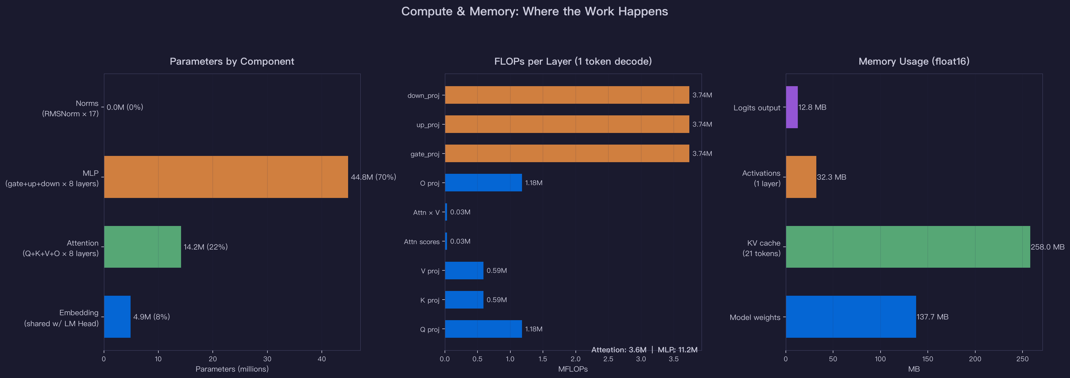
Parameters (left): The MLP dominates at 70% — this is where knowledge is stored. Attention is 22%. The embedding/LM head is 8% (shared via weight tying, counted once).

FLOPs per layer (middle): For a single decode step, the MLP projections (gate, up, down) dominate. Attention score computation scales with sequence length, but for short sequences the MLP is the bottleneck.

Memory (right): Model weights dominate at 138MB (float16). KV cache and activations are tiny for this model — but they grow with sequence length and become the primary concern for larger models.

---

Summary: The Complete Data Flow

"What is AI?"
     │
     ▼ Tokenizer
[1, 832, 311, 234, 1146, 395, 1891, 66, 2, ...]  ← 21 integers
     │
     ▼ Embedding [6400 × 768] — row lookup
[21 × 768] float vectors                           ← each token is now 768 numbers
     │
     ▼ ×8 Transformer Layers, each:
     │   ├── RMSNorm [768 weights]
     │   ├── Attention: Q[768×768] K[768×384] V[768×384] O[768×768]
     │   │   └── 8 heads × softmax(QK^T/√96) × V
     │   ├── + Residual
     │   ├── RMSNorm [768 weights]  
     │   ├── SwiGLU: gate[2432×768] up[2432×768] down[768×2432]
     │   │   └── down(SiLU(gate(x)) × up(x))
     │   └── + Residual
     │
     ▼ Final RMSNorm
[21 × 768]                                         ← refined representations
     │
     ▼ LM Head [6400 × 768] — matrix multiply  
[6400] logits                                       ← one score per vocabulary word
     │
     ▼ ÷ temperature → softmax → top-p filter → sample
"AI"                                                ← one token chosen
     │
     └── Append to input, repeat until EOS

All the “intelligence” — language understanding, factual knowledge, reasoning — is encoded in 64 million floating-point numbers spread across 91 weight tensors (some shared via weight tying). Training adjusted these numbers across millions of text examples so that, given any sequence of tokens, the model assigns high probability to the correct next token.

There is no database lookup, no rule engine, no knowledge graph. Just matrix multiplications, nonlinear activations, and a softmax at the end. And yet, the model answers: “AI is…”

---

Try It Yourself

The complete runnable walkthrough script and all visualization code are available:

• Model: MiniMind-3 (64M params, Apache 2.0)
• Weights: HuggingFace
• Dataset: HuggingFace

Run inference on a Mac (MPS), CUDA GPU, or even CPU:

cd minimind
python eval_llm.py --device mps --weight full_sft

The model is small enough to train from scratch in ~8 hours on an M3 Mac or ~2 hours on a 3090.

---

Self-Check

1. If the vocabulary were 100K instead of 6,400, how would the embedding table and LM head sizes change? What about inference speed?
2. Why does the MLP have 65% of the parameters but the attention mechanism is considered the “harder” infrastructure challenge?
3. Why does the causal mask set the upper-right triangle to $-\infty$ instead of zero?
4. If top-p = 1.0 and temperature = 0, what sampling strategy does that reduce to?
5. The model has 8 attention heads but only 4 KV heads (GQA). What’s the memory saving for KV cache at sequence length 4096?

---

References

1. Vaswani et al., “Attention Is All You Need” (2017) — Original transformer architecture
2. Shazeer, “GLU Variants Improve Transformer” (2020) — SwiGLU activation
3. Su et al., “RoFormer: Enhanced Transformer with Rotary Position Embedding” (2021) — RoPE
4. Ainslie et al., “GQA: Training Generalized Multi-Query Transformer Models” (2023) — Grouped-Query Attention
5. Holtzman et al., “The Curious Case of Neural Text Degeneration” (2020) — Top-p (nucleus) sampling
6. MiniMind GitHub — The model used in this article