MoE Inference Visualized — How Expert Routing Actually Works Inside a Real Model
TL;DR
Mixture-of-Experts (MoE) changes exactly one thing in the transformer inference pipeline: it replaces the single feed-forward MLP with multiple expert MLPs and a tiny router that assigns each token to one expert. Everything else — tokenization, embedding, attention, sampling — is identical. We visualize the router decisions, expert execution, and load balancing using a real 198M-parameter MoE model, compared side-by-side with its 64M dense counterpart.
Prerequisite: This article builds on Visualizing Every Step of LLM Inference, which walks through the complete dense inference pipeline. We won’t repeat those steps here — only the parts that MoE changes.
What MoE Changes — and What It Doesn’t
In a standard (dense) transformer, every token passes through the same MLP in each layer. In an MoE transformer, that single MLP is replaced by multiple copies (experts), and a router decides which expert each token uses.
Here’s the side-by-side comparison of a single layer:
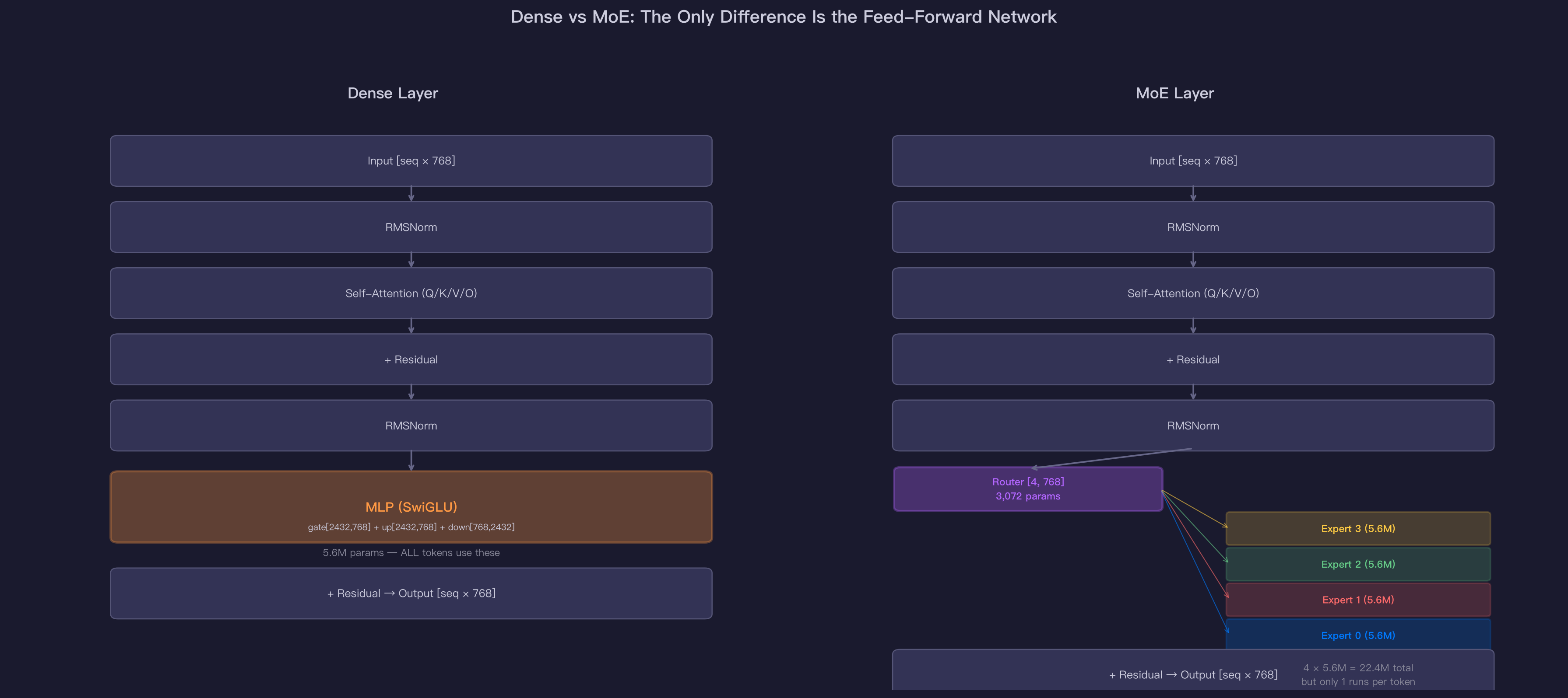
Left (Dense): One MLP with 5.6M parameters. Every token uses the same weights.
Right (MoE): A tiny router (3,072 parameters) plus 4 expert MLPs (5.6M each = 22.4M total). Each token is routed to exactly one expert. The computation per token is the same — only the weights differ.
Everything outside the dashed area is identical between dense and MoE:
| Component | Dense | MoE | Different? |
|---|---|---|---|
| Tokenization | ✓ | ✓ | No |
| Embedding lookup | [6400, 768] | [6400, 768] | No |
| RMSNorm | [768] | [768] | No |
| Self-Attention (Q/K/V/O) | Same | Same | No |
| Residual connections | Same | Same | No |
| Feed-Forward (MLP) | 1 MLP | Router + 4 expert MLPs | Yes |
| LM Head | [6400, 768] | [6400, 768] | No |
| Sampling (temperature, top-p) | Same | Same | No |
The Router: 3,072 Parameters That Control Everything
The router is a single linear layer — shape [4, 768] — that maps each token’s 768-dimensional hidden state to 4 scores (one per expert). Softmax turns these scores into probabilities, and the top-1 expert is selected.
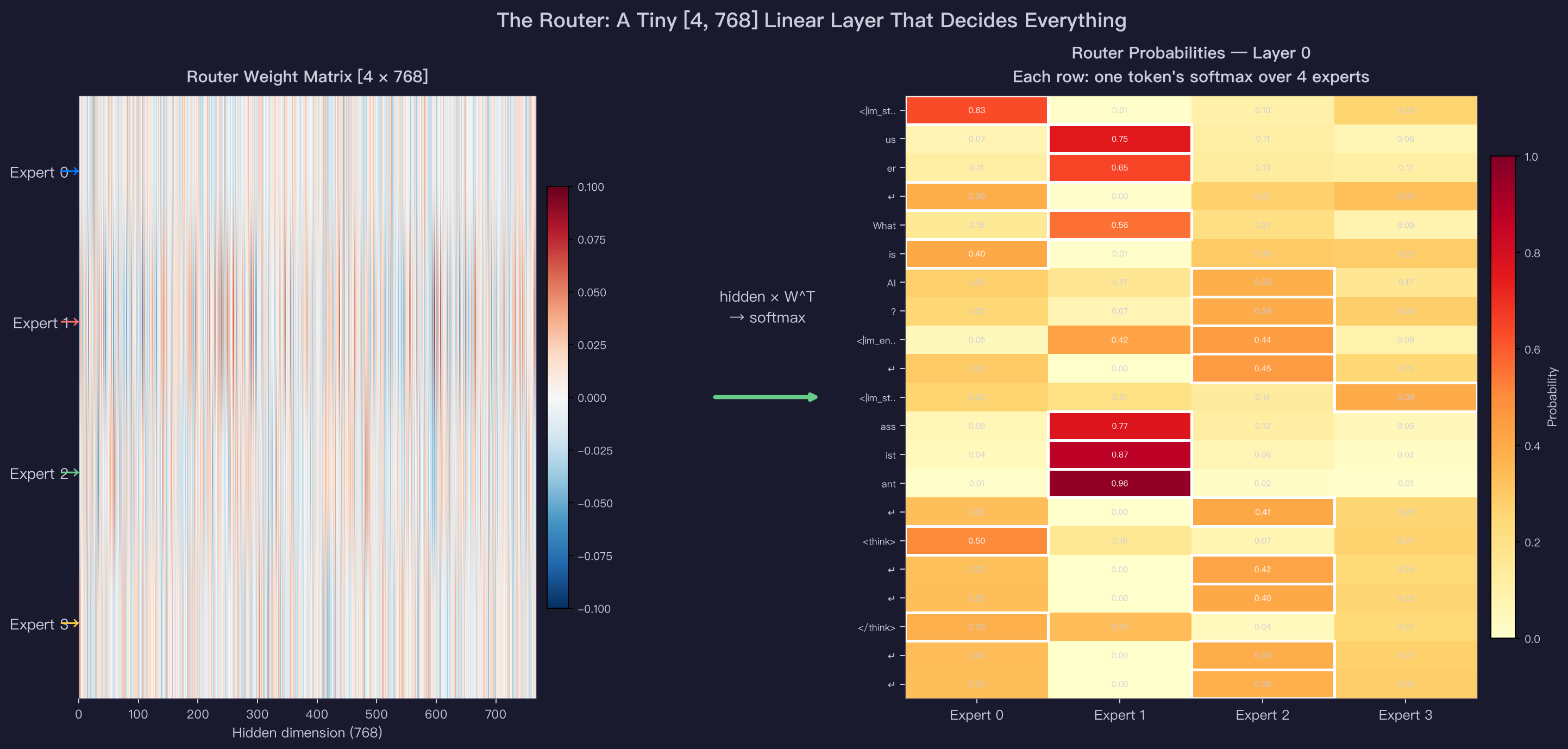
Left: The actual router weight matrix from Layer 0. Each of the 4 rows is a 768-dimensional vector that defines what “kind” of token each expert prefers. The dot product between a token’s hidden state and each row determines the routing.
Right: The resulting probabilities for each token in our prompt “What is AI?” White boxes mark the chosen expert. Notice:
- “us”, “er”, “What”, “ass”, “ist”, “ant” → Expert 1 (high confidence, 0.56–0.96). These are common subword tokens — Expert 1 appears to specialize in basic vocabulary.
- ” AI”, ”?”,
<|im_end|>→ Expert 2. Content tokens and punctuation. <|im_start|>, ” is”,<think>,</think>→ Expert 0. Structural and function words.- Only one token goes to Expert 3 this layer.
The router computation is trivial:
With 3,072 parameters (0.01% of the model), the router is essentially free in both compute and memory.
Token-to-Expert Assignment
Each token is assigned to exactly one expert. Here’s the mapping for Layer 0:
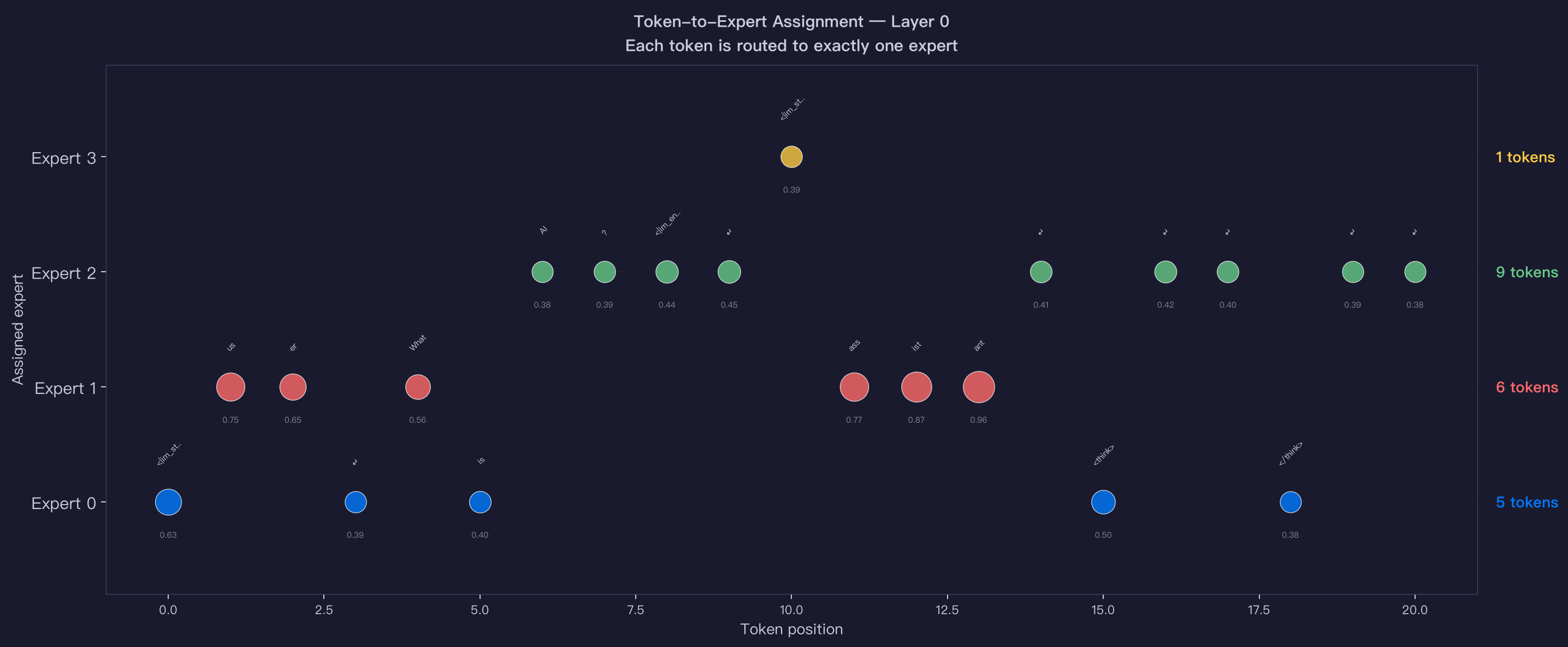
Each dot is a token, positioned at its assigned expert. The dot size represents the router’s confidence (larger = higher softmax probability). The numbers below each dot show the exact router weight.
Key observations:
- Expert 1 gets 6 tokens with high confidence (0.55–0.96) — the router is very sure about these assignments.
- Expert 0 gets 5 tokens but with lower confidence (0.38–0.63) — the router is less certain.
- Expert 3 gets only 1 token — severe underutilization in this layer.
Routing Across All 8 Layers
The same token can be routed to different experts in different layers. The router weights are independent per layer, so a token that goes to Expert 0 in Layer 2 might go to Expert 2 in Layer 5:
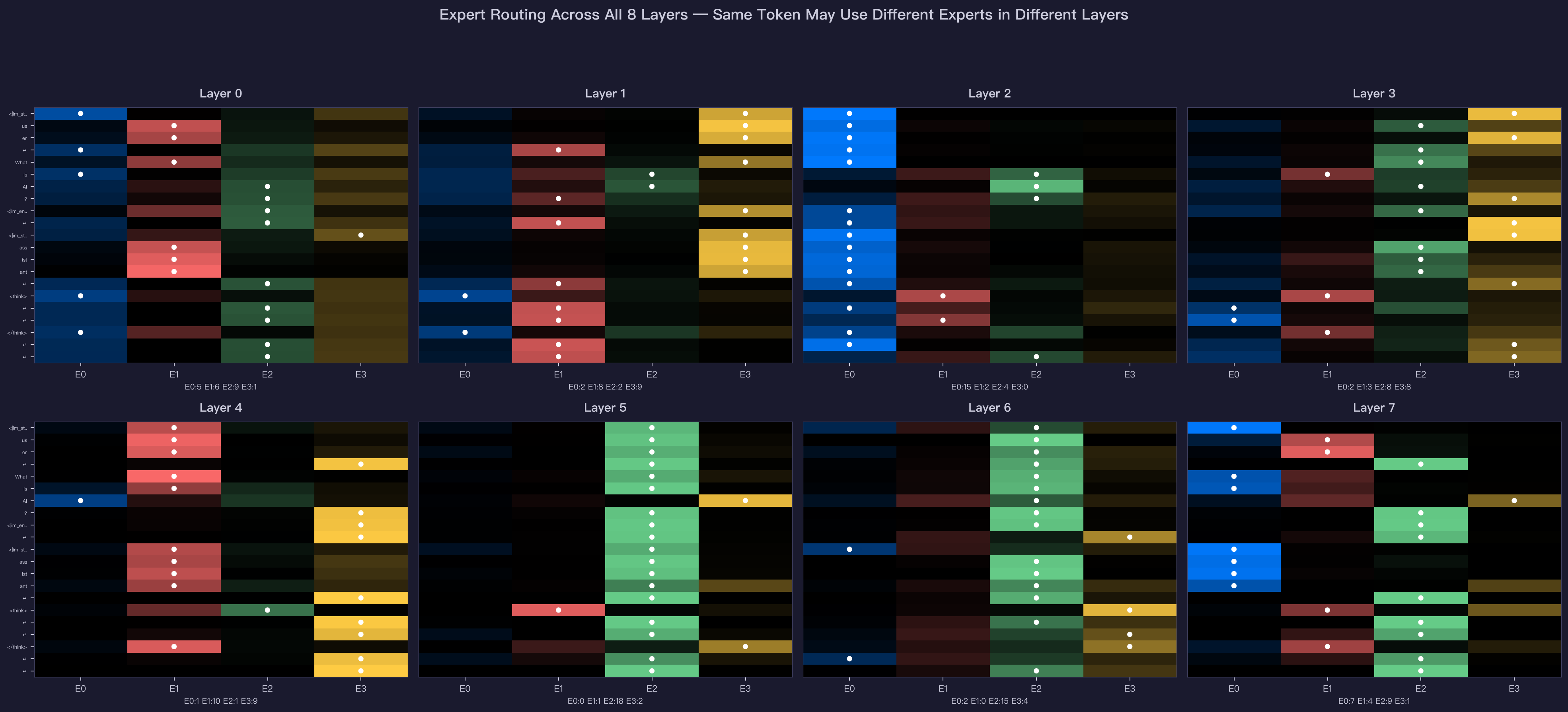
Each panel shows one layer. The white dots (●) mark the chosen expert for each token. The background color intensity shows the router probability — brighter means higher confidence.
Notice:
- Layer 2: Expert 0 dominates with 15 out of 21 tokens — massive imbalance.
- Layer 5: Expert 2 handles 18 tokens (86%!) — even more extreme.
- Layer 7: More balanced distribution across experts.
- No single token uses the same expert in all layers — the routing is genuinely dynamic.
Load Balance: The MoE Challenge
Ideally, each expert would handle 25% of tokens (5.25 out of 21). In practice, the distribution is often heavily skewed:
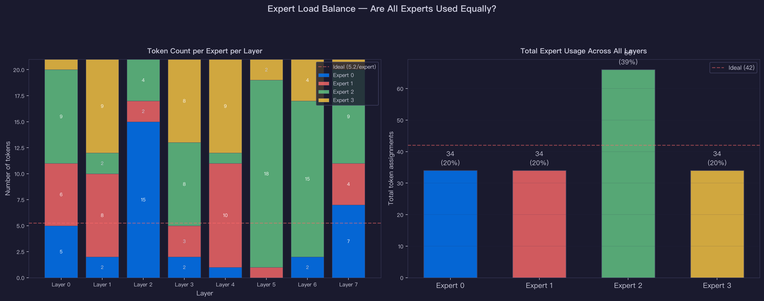
Left: Per-layer breakdown. The red dashed line shows the ideal even split. Several layers deviate dramatically — Layer 5 sends 86% of tokens to a single expert.
Right: Aggregated across all layers. Expert 2 handles 39% of all routing assignments, while Experts 0, 1, and 3 each handle about 20%.
This imbalance matters for two reasons:
- Wasted capacity: Expert 3 has 5.6M parameters but only processes 20% of tokens. Those parameters are underutilized.
- Infrastructure bottleneck: In distributed setups where experts live on different GPUs, one GPU becomes a bottleneck while others idle.
This is why MoE training uses an auxiliary loss (router_aux_loss_coef = 0.0005 in this model) — a penalty term that encourages the router to distribute tokens more evenly. But as we can see, perfect balance remains difficult.
Expert Execution: Gather → Compute → Scale → Scatter
Once the router assigns tokens, execution happens in four steps:
- Gather: Collect all tokens assigned to each expert
- Compute: Run that expert’s MLP (identical to a dense MLP — gate/up/down projections)
- Scale: Multiply the output by the router weight (the softmax probability)
- Scatter: Put results back into the correct sequence positions
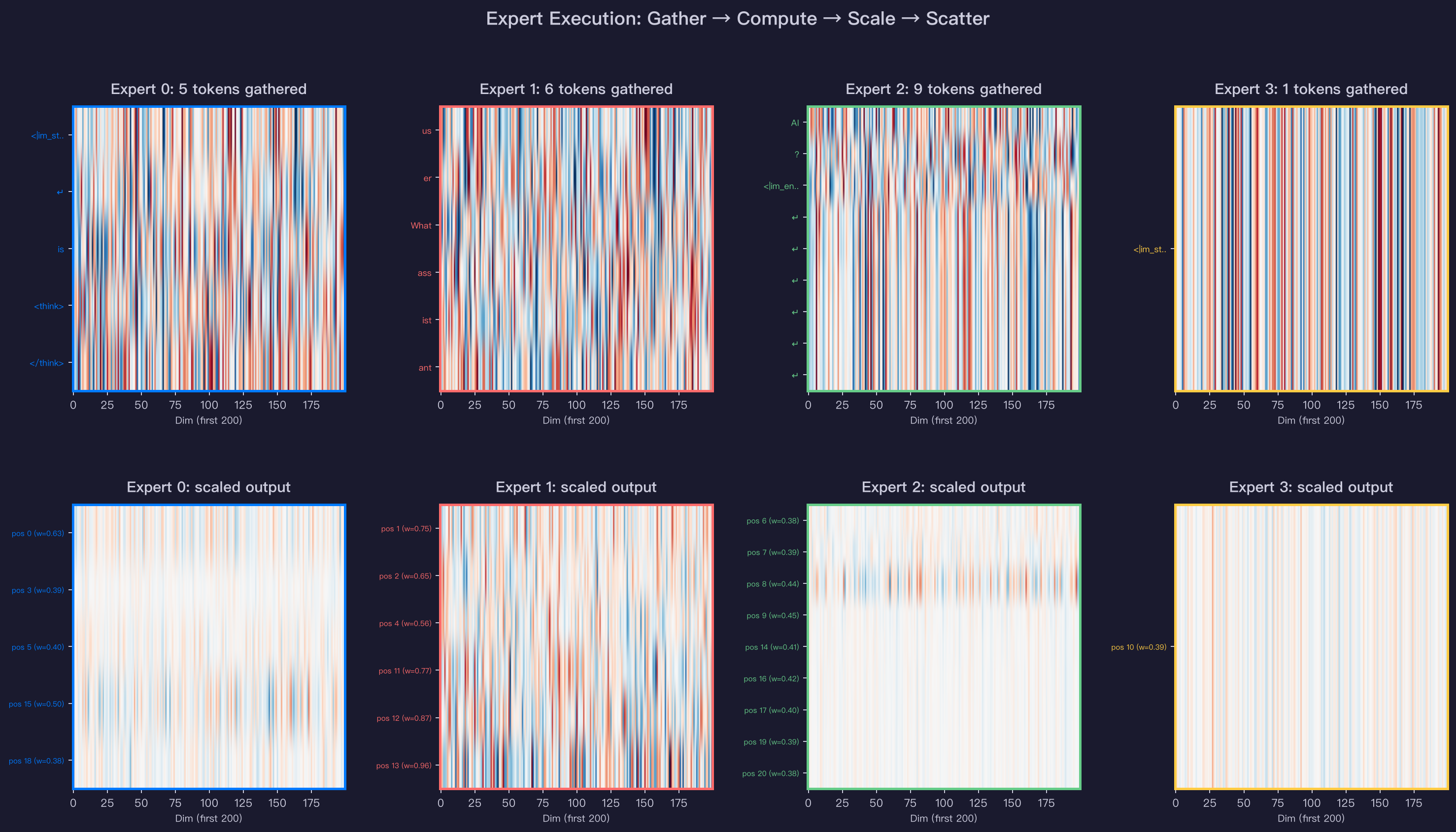
Top row: The input tensors gathered for each expert. Notice they have different numbers of rows — Expert 1 has 6 tokens, Expert 3 has only 1.
Bottom row: The scaled output. Each expert’s output is multiplied by its router weight before scattering back. This scaling means a token routed to an expert with 95% confidence gets nearly the full expert output, while a token routed with 38% confidence gets a dampened version.
The computation inside each expert is exactly the same as the dense MLP:
expert_output = down_proj(SiLU(gate_proj(input)) × up_proj(input))
final_output = expert_output × router_weight
No special MoE math — just a regular SwiGLU MLP with a scalar multiplier.
Router Confidence: How Sure Are the Routing Decisions?
The router’s softmax probability for the chosen expert tells us how “confident” the routing is:
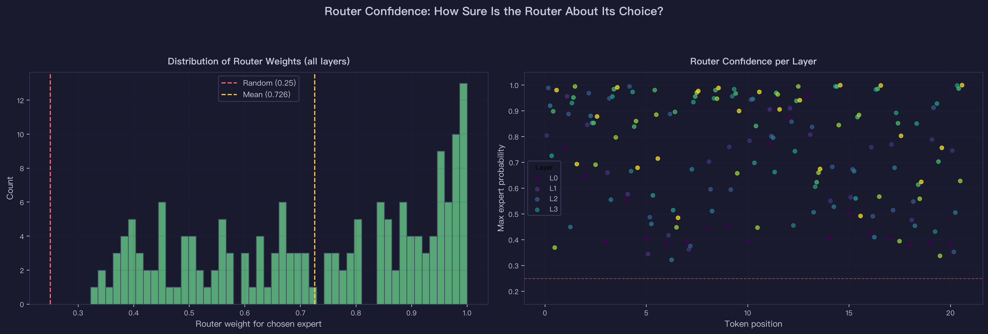
Left: Distribution of router weights across all layers and tokens. The peak is around 0.35–0.45, well above the random baseline of 0.25 (red dashed line). Some tokens are routed with 96% confidence, while others are near 30% — barely better than random.
Right: Per-token confidence across layers. Some tokens (like “ant” in certain layers) consistently get high-confidence routing, while structural tokens (newlines, special tokens) tend to get lower confidence — the router is less sure where they “belong.”
Low-confidence routing means the token would get a similar result from multiple experts — suggesting those experts have overlapping specializations.
The Tradeoff: Parameters vs Memory vs Compute
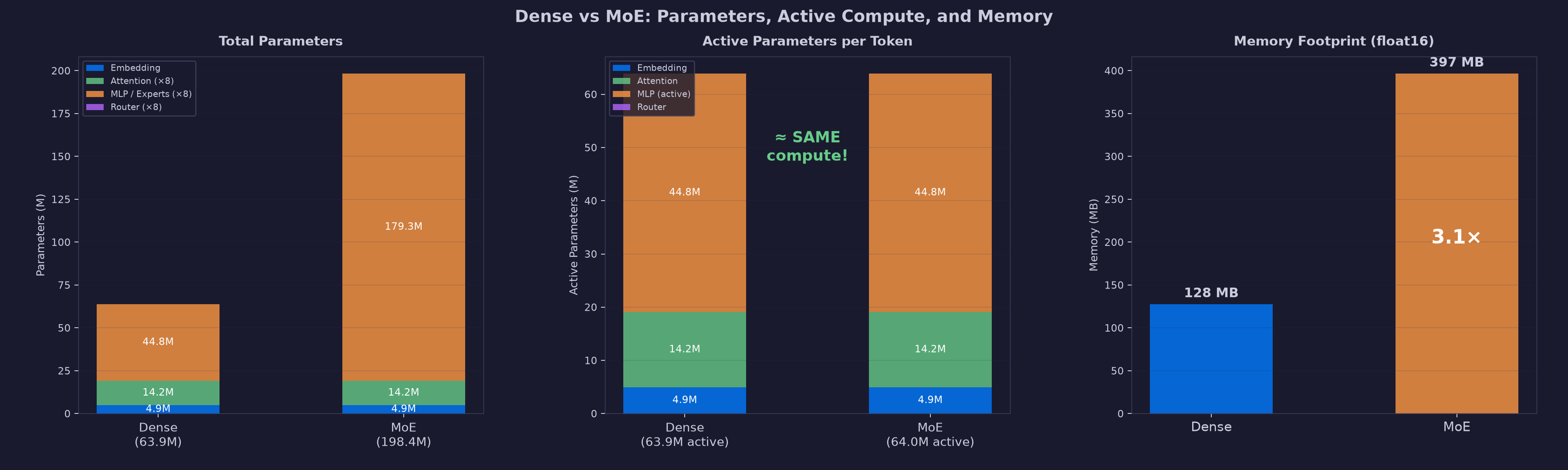
The three panels tell the complete MoE story:
Total Parameters (left): MoE has 198M parameters — 3.1× more than dense (64M). The extra parameters are entirely in the replicated expert MLPs.
Active Parameters per Token (middle): Only 64M parameters are active per token — the same as the dense model! The router selects one expert, so only one expert’s MLP weights are used per token. The FLOPs are identical.
Memory (right): MoE requires 397 MB to store all expert weights in float16, compared to 128 MB for dense. All expert weights must be in memory even though only one runs per token.
| Metric | Dense | MoE (4 experts, top-1) |
|---|---|---|
| Total parameters | 63.9M | 198.4M (3.1×) |
| Active parameters / token | 63.9M | ~64.0M (same) |
| FLOPs / token | F | F (same) |
| Memory (float16) | 128 MB | 397 MB (3.1×) |
| MLP parameters / layer | 5.6M | 22.4M (4×) |
| Active MLP / token | 5.6M | 5.6M (same) |
| Router overhead | — | 3,072 params (negligible) |
The fundamental tradeoff: MoE trades memory for capacity. You get 3× more knowledge storage for the same compute cost per token, but you must keep all expert weights in memory (or manage expert parallelism across GPUs).
Why MoE Matters for Infrastructure
MoE creates unique infrastructure challenges that don’t exist for dense models:
Expert parallelism: With large MoE models (like Mixtral-8×7B or DeepSeek-V3), experts are spread across GPUs. Each token’s routing decision triggers an all-to-all communication — tokens must be sent to whichever GPU holds their selected expert, then results sent back. This communication pattern is fundamentally different from tensor or pipeline parallelism.
Load imbalance: As we saw, some experts handle 86% of tokens while others sit idle. This creates GPU utilization imbalance — one GPU is the bottleneck while others wait. Solutions include auxiliary loss penalties, capacity factors (dropping tokens that exceed an expert’s buffer), and expert-choice routing (experts pick tokens instead of tokens picking experts).
Memory vs compute disconnect: MoE models are memory-bandwidth-bound during inference because they store 3–8× more weights but only activate a fraction per token. The arithmetic intensity drops compared to dense models, making MoE particularly sensitive to memory bandwidth.
KV cache is unchanged: Since attention is identical in MoE and dense, the KV cache behavior is the same. This means MoE inference optimizations can focus entirely on the MLP execution path.
Summary
Dense inference:                    MoE inference:

 token → MLP → output               token → Router (3K params)
         ↑                                    │
    5.6M params                               ▼
    ALL tokens use same             ┌─ Expert 0 (5.6M) ← some tokens
                                    ├─ Expert 1 (5.6M) ← some tokens
                                    ├─ Expert 2 (5.6M) ← some tokens
                                    └─ Expert 3 (5.6M) ← some tokens

                                    Only the selected expert runs.
                                    Same compute as dense.
                                    3× more stored knowledge.
                                    3× more memory.
MoE is not a fundamentally different architecture — it’s a conditional computation trick applied to the MLP. The same SwiGLU computation runs, but different tokens use different weight matrices. A tiny router (0.01% of model parameters) makes all the routing decisions.
The result: models that are much larger on paper but run at the same speed — provided you have enough memory to hold all the expert weights.
Self-Check
- If you increase from 4 experts to 8 experts (still top-1), how do total parameters, active parameters, and memory change?
- What happens if top-k = 2 instead of top-1? How does that affect compute and output quality?
- Why does the auxiliary loss help with load balancing? What would happen without it?
- In a distributed setup with 4 GPUs (one expert per GPU), what communication pattern does MoE require compared to tensor parallelism?
- Looking at the routing patterns, Layer 5 sends 86% of tokens to Expert 2. Is this necessarily bad? When might extreme specialization be beneficial?
References
- Shazeer et al., “Outrageously Large Neural Networks: The Sparsely-Gated Mixture-of-Experts Layer” (2017) — Original MoE for transformers
- Fedus et al., “Switch Transformers: Scaling to Trillion Parameter Models with Simple and Efficient Sparsity” (2022) — Top-1 routing, simplified MoE
- Jiang et al., “Mixtral of Experts” (2024) — Mixtral-8×7B, demonstrating MoE at production scale
- DeepSeek-AI, “DeepSeek-V3 Technical Report” (2024) — 671B MoE with auxiliary-loss-free load balancing
- MiniMind GitHub — The model used in this article
- Visualizing Every Step of LLM Inference — The companion dense model article