Visualizing Every Step of LLM Training — How 64M Parameters Learn to Predict Text

TL;DR

Training is inference in reverse. The forward pass is identical — but instead of sampling a token, we compute how wrong the prediction was (loss), propagate that error backwards through every layer (backpropagation), and nudge every weight to make the prediction slightly better (optimizer step). We visualize each of these steps using real gradients from a 64M-parameter transformer.

Prerequisite: This article builds on Visualizing Every Step of LLM Inference. The forward pass is the same — we focus here on what training adds: loss, gradients, and weight updates.

---

What Training Adds to Inference

Inference runs the model forward and samples a token. Training runs the same forward pass, but then adds three more steps:

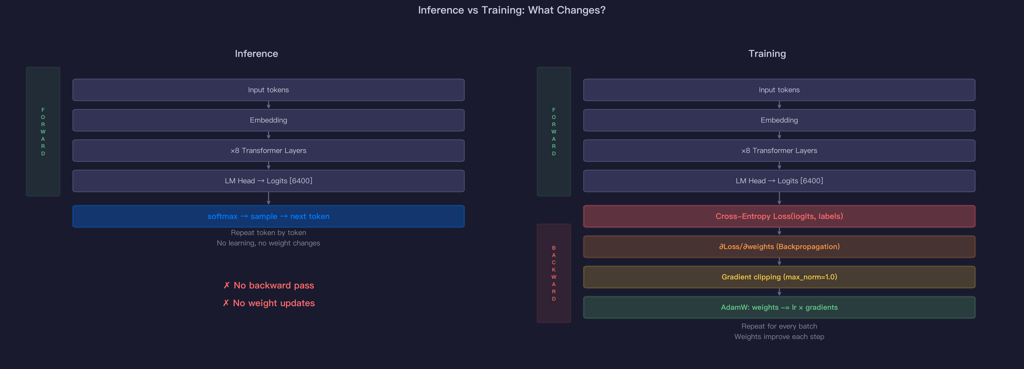
Left (Inference): Forward pass → softmax → sample next token. Weights are frozen — the model doesn’t learn.

Right (Training): Forward pass → compute loss → backpropagate gradients → clip gradients → update weights with optimizer. Each step modifies the model to make better predictions next time.

The forward pass is identical. Everything that follows is new.

---

Step 1: The Training Objective — Predict the Next Token

The model’s entire training objective is simple: given a sequence of tokens, predict the next token at every position. The labels are just the input shifted by one position:

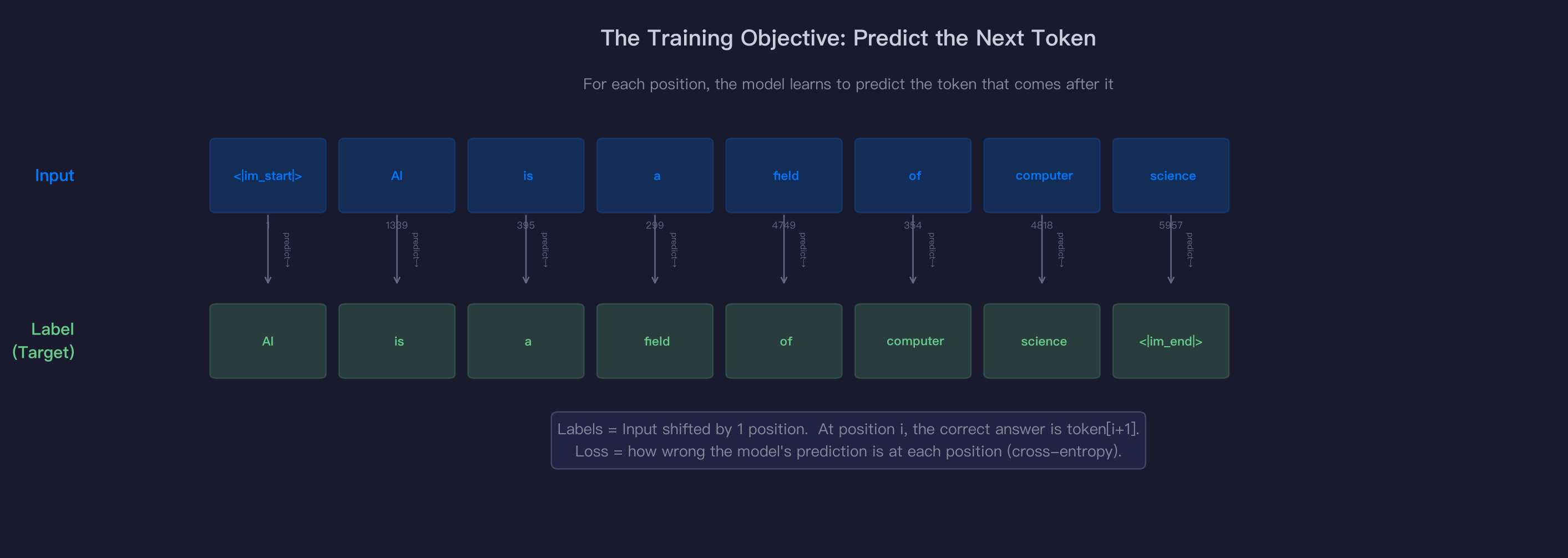
At position $i$, the input is token $i$, and the correct answer (label) is token $i+1$. The model learns by being told “you predicted X, but the answer was Y” at every position simultaneously.

This is why language models are so data-efficient — a single sentence of $n$ tokens provides $n-1$ training examples, all processed in one forward pass.

---

Step 2: Pretrain vs SFT — Which Tokens Count?

The training objective is the same for both pretraining and SFT, but they differ in which tokens the model learns from:

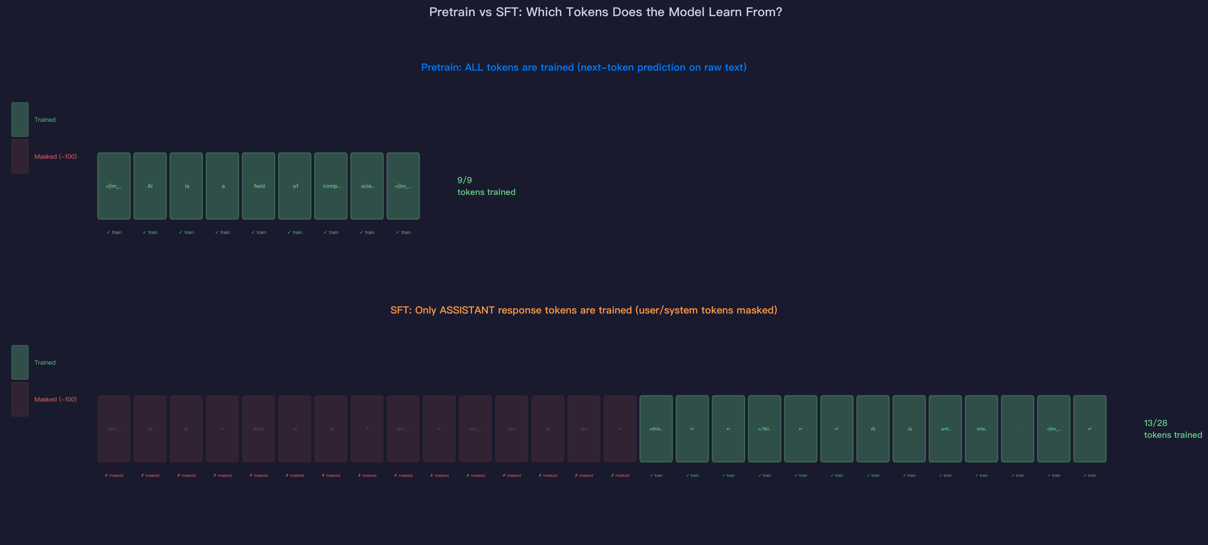
Pretrain (top): Every token in the sequence is a training target. The model learns to predict all text — grammar, facts, reasoning patterns. All 9 tokens contribute to the loss.

SFT (bottom): Only the assistant’s response tokens contribute to the loss. User messages, system prompts, and special tokens are masked with label -100 (PyTorch’s convention for “ignore this position”). Out of 28 tokens, only 13 are trained on.

The masking is implemented in the dataset, not the model — labels of -100 are simply excluded from the loss calculation. The forward pass still processes all tokens (attention needs the full context), but gradients only flow from the unmasked positions.

This is why SFT teaches the model to respond rather than to parrot user messages — it only gets credit for the assistant’s output.

	Pretrain	SFT
Data	Raw text	Conversations
Trained tokens	All	Assistant only
Label for user tokens	Next token	-100 (masked)
Learning rate	5e-4 (high)	1e-5 (50× lower)
Starting weights	Random	Pretrained
Goal	Learn language	Learn to assist

---

Step 3: Cross-Entropy Loss — Measuring How Wrong the Prediction Is

At each position, the model outputs 6,400 logits (one per vocabulary word). The cross-entropy loss measures how wrong the prediction is by looking at the probability assigned to the correct token:

$$\text{Loss}_i = -\log P(\text{correct token at position } i)$$

If the model assigns 95% probability to the right token → loss ≈ 0.05 (good). If the model assigns 1% → loss ≈ 4.6 (bad). If the model assigns 0.01% → loss ≈ 9.2 (terrible).

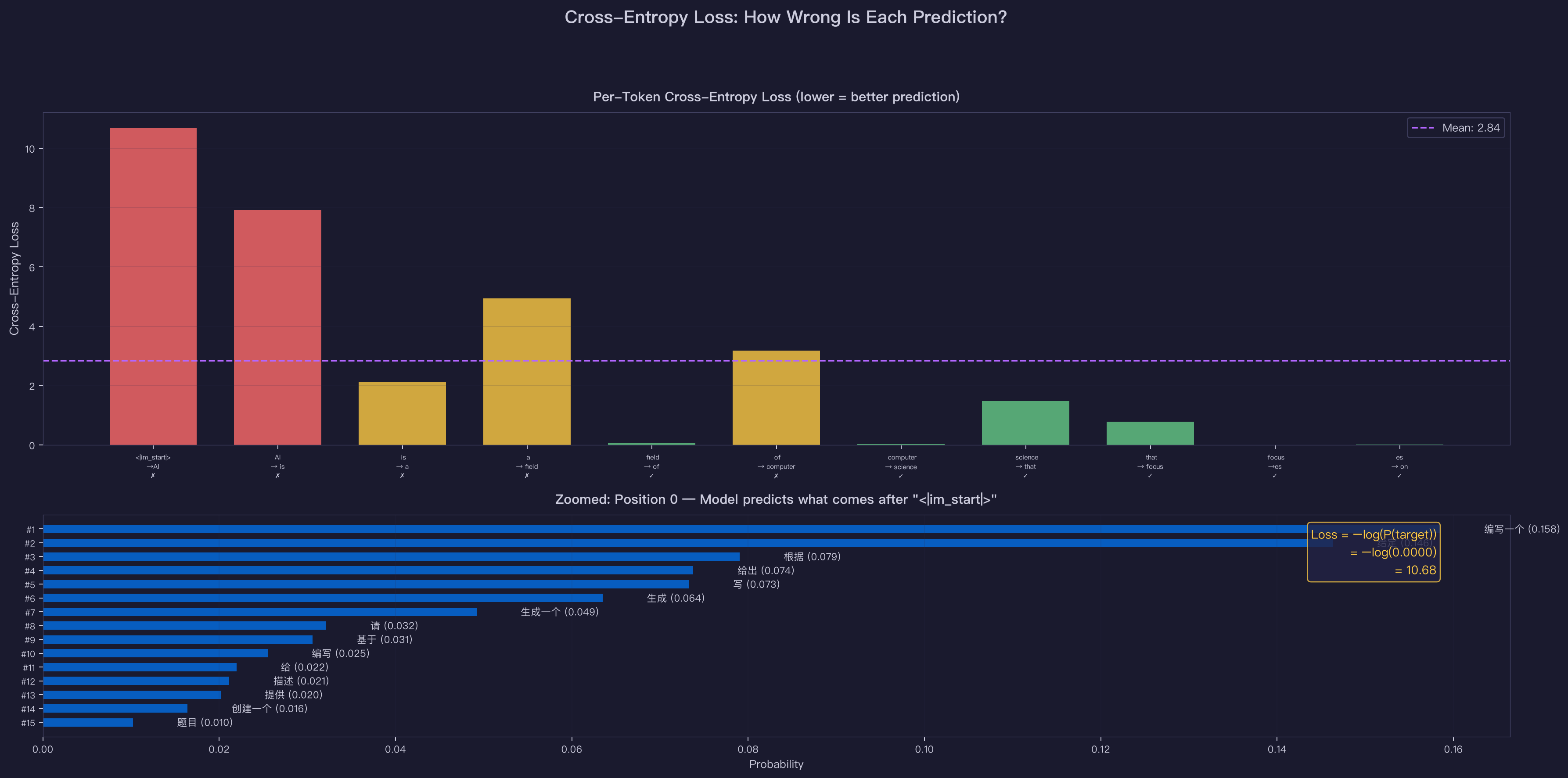
Top: Per-token loss for the sentence “AI is a field of computer science that focuses on”. Green bars = low loss (model predicted correctly). Red bars = high loss (model was wrong). Each position shows the input token, the target, and whether the model’s top prediction matched (✓/✗).

Bottom: Zoomed into position 0 — the model’s probability distribution over all 6,400 words. The target token and its probability are highlighted. The formula box shows how the scalar loss is computed from this single probability.

The total loss is the average across all unmasked positions:

$$\text{Loss} = \frac{1}{N} \sum_{i=1}^{N} -\log P(y_i \mid x_1, \ldots, x_i)$$

This single number — one scalar — is what drives the entire learning process. Every gradient, every weight update, every improvement traces back to reducing this number.

---

Step 4: Backpropagation — Tracing the Error Backwards

The loss tells us how wrong the model is. Backpropagation tells us which weights are responsible and in which direction to adjust them.

Starting from the loss, the chain rule of calculus propagates gradients backwards through every operation — from the LM head, through all 8 transformer layers, down to the embedding table. Each weight receives a gradient: ∂Loss/∂weight.

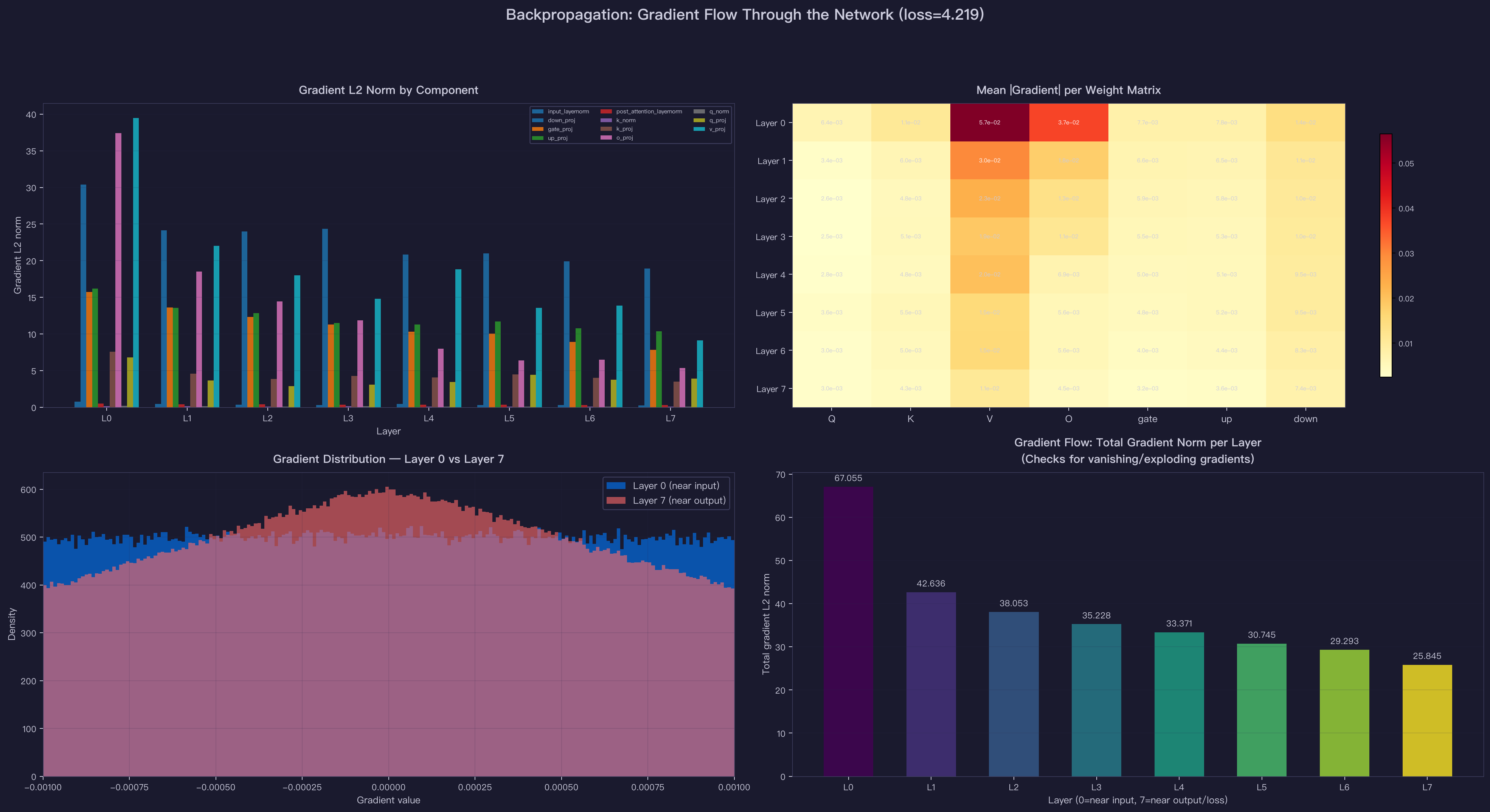
Four views of the actual gradients from one training step:

Top-left: Gradient L2 norm by component per layer. Layer 0 has the largest gradients despite being farthest from the loss. This is because residual connections create a “gradient highway” — each residual addition accumulates gradients, so earlier layers receive contributions from all subsequent residual paths.

Top-right: Mean |gradient| heatmap. Each cell shows the average gradient magnitude for one weight matrix in one layer. The V projection in Layer 0 has the hottest gradient — residual accumulation concentrates gradient signal in the earlier layers.

Bottom-left: Gradient distribution. Layer 0 (blue, near input) has a wider gradient distribution than Layer 7 (red, near output). Despite being farther from the loss, Layer 0 receives accumulated gradients through all 8 residual connections — each residual output = input + f(input) splits the gradient, sending a copy straight through to earlier layers.

Bottom-right: Total gradient norm per layer. Layer 0 has the highest gradient norm (67.1), decreasing to Layer 7 (25.8) — a 2.6× difference. This pattern (higher gradients for earlier layers) is the opposite of what you’d see without residual connections. In a plain deep network, gradients vanish in earlier layers. Here, residual connections reverse this: they create shortcut paths that carry gradient signal directly to early layers, accumulating across all 8 residual additions.

Why This Matters for Infrastructure

Backpropagation is the most memory-intensive phase of training. During the forward pass, every intermediate activation must be saved for the backward pass (because the chain rule needs them). For a 64M model this is manageable, but for billion-parameter models, activation memory dominates — leading to techniques like gradient checkpointing, activation offloading, and ZeRO optimization.

---

Step 5: Weight Updates — Nudging 64 Million Numbers

After backpropagation, every weight has a gradient. The optimizer uses these gradients to adjust the weights. But first — gradient clipping.

Gradient Clipping

If gradients become too large, the weight update can be catastrophically big — destroying what the model has already learned. Gradient clipping computes the total L2 norm across all parameters and rescales if it exceeds a threshold:

$$\text{if } \|\nabla\| > \text{max\_norm}: \quad \nabla \leftarrow \nabla \times \frac{\text{max\_norm}}{\|\nabla\|}$$

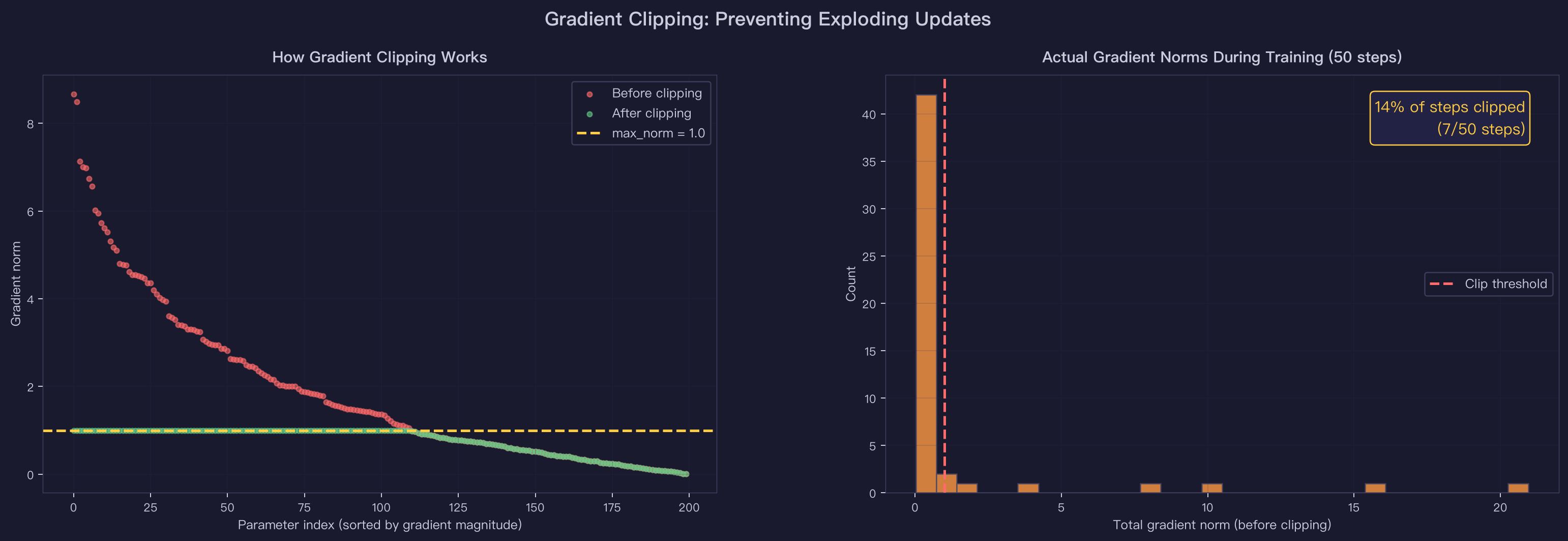
Left: The concept — all gradients above the threshold are scaled down proportionally. Right: Actual gradient norms from 50 training steps. Many steps exceed the clip threshold of 1.0, especially early in training when the model is making large errors.

The Optimizer Step

After clipping, AdamW applies the update. For each weight:

1. Compute exponential moving average of gradients (momentum)
2. Compute exponential moving average of squared gradients (adaptive learning rate)
3. Update: weight -= lr × momentum / (√variance + ε) + weight decay

The result is a tiny adjustment to each of the 64 million parameters:

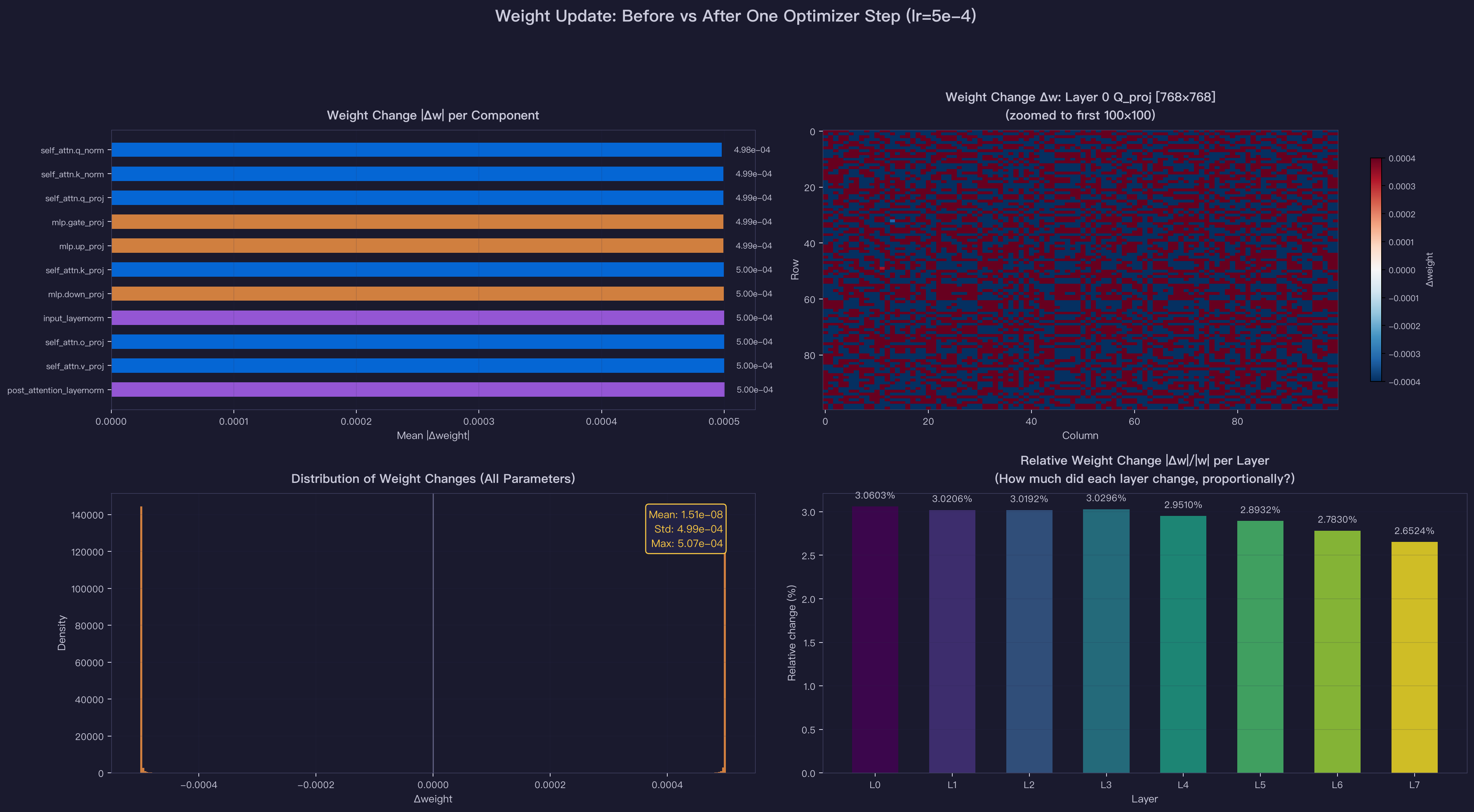
Top-left: Weight change per component. MLP projections receive the largest updates, followed by attention projections. Norms change the least.

Top-right: Actual weight change heatmap. The Δw matrix for Layer 0’s Q projection — each pixel is one weight’s change. The pattern is sparse and structured, not random.

Bottom-left: Distribution of all weight changes. Centered at zero with standard deviation ~10⁻⁴. Most weights barely change — but across millions of weights and thousands of steps, these tiny changes accumulate into a model that predicts language.

Bottom-right: Relative change per layer. Each layer changes by about 0.003–0.006% of its total weight magnitude per step. Layer 0 changes the most (it receives the largest accumulated gradients via residual connections), Layer 7 the least.

---

Step 6: Learning Rate Schedule — Controlling Update Size

The learning rate determines how big each weight update is. Too high → unstable, weights oscillate. Too low → learning is painfully slow.

MiniMind uses a cosine decay schedule:

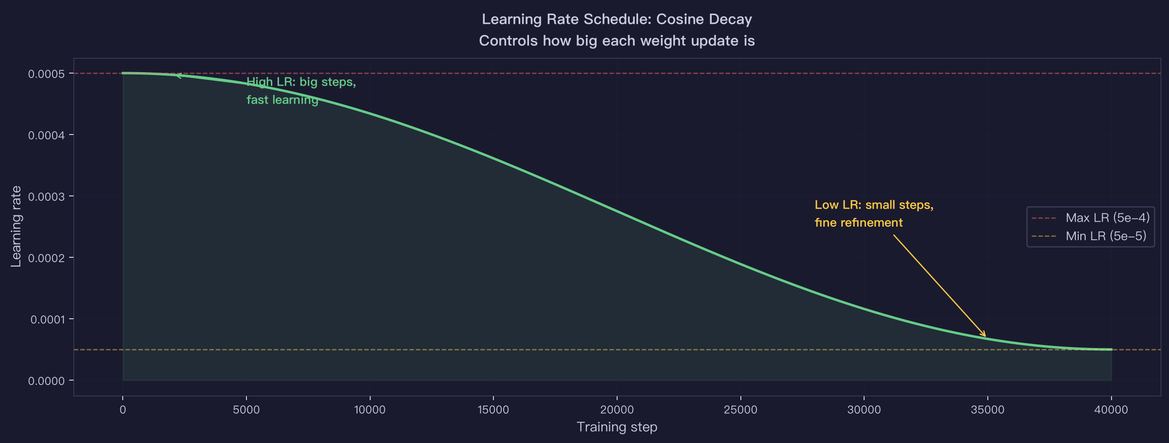
The learning rate starts high (5×10⁻⁴) for fast initial learning, then gradually decays following a cosine curve to a minimum of 5×10⁻⁵. This matches the training dynamics:

• Early training: The model knows nothing — big updates needed to learn basic patterns.
• Late training: The model already knows most patterns — small updates for fine refinement without disrupting what’s learned.

For SFT, the peak learning rate is 50× lower (1×10⁻⁵) because the pretrained model already knows language — we’re fine-tuning, not learning from scratch.

---

Step 7: Watching the Model Learn — 50 Steps from Random

Finally, let’s watch a model learn in real time. Starting from random weights, we train for 50 steps on a small batch:

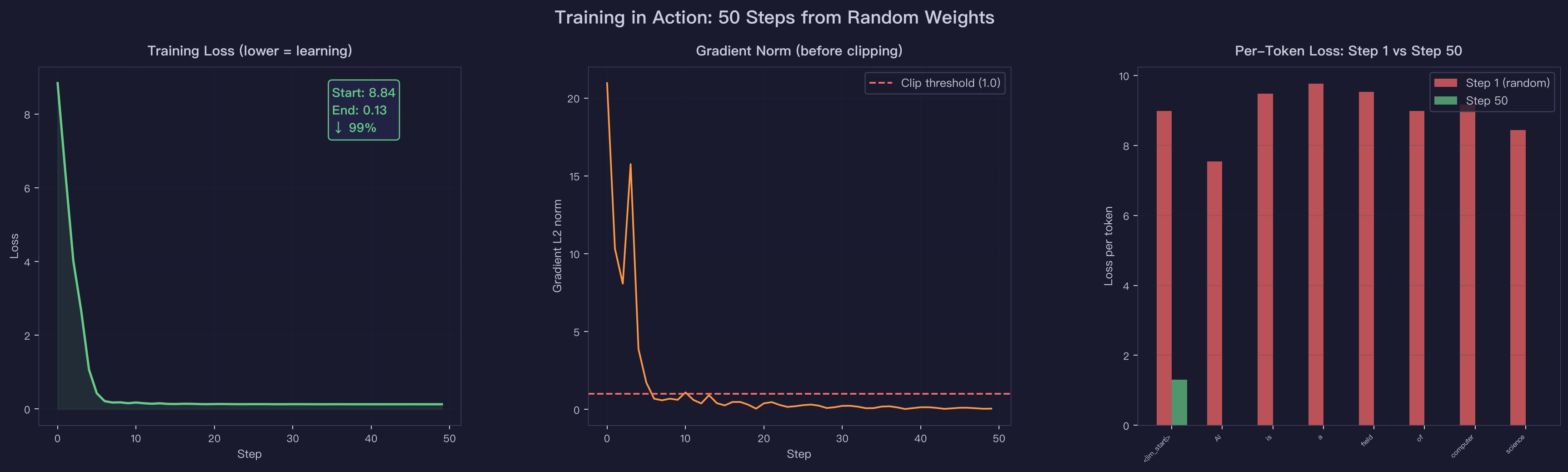
Left: Loss curve. Loss drops rapidly in the first 10 steps, then gradually levels off. The model goes from random guessing (loss ≈ 8.7, close to $-\log(1/6400) = 8.76$) to meaningful predictions in just 50 steps.

Middle: Gradient norm. Initially very high (the model is wildly wrong), gradually settling down as the model improves. The red line shows the clip threshold — early steps are heavily clipped.

Right: Per-token loss before and after. Red bars show loss at step 1 (random model) — uniformly high. Green bars show loss at step 50 — dramatically lower for most tokens. The model has started learning which tokens follow which.

---

The Complete Training Loop

Putting it all together — this is what repeats for every batch, for every epoch:

For each batch of training data:
    
    1. FORWARD PASS (same as inference)
       tokens → embedding → 8 × (attention + MLP) → LM head → logits
    
    2. COMPUTE LOSS
       loss = cross_entropy(logits[:-1], labels[1:])    # shifted by 1
       loss = mean over unmasked positions               # pretrain: all, SFT: assistant only
    
    3. BACKWARD PASS  
       loss.backward()                                   # chain rule through every layer
       → every weight gets ∂loss/∂weight                 # ~64M gradients computed
    
    4. GRADIENT CLIPPING
       if total_gradient_norm > 1.0:                     # prevent exploding updates
           scale all gradients by 1.0 / total_norm
    
    5. OPTIMIZER STEP (AdamW)
       for each weight:
           weight -= lr × adjusted_gradient              # tiny nudge, ~0.004% change
       
    6. ZERO GRADIENTS
       optimizer.zero_grad()                             # reset for next batch
    
    Repeat ~40,000 times (1 epoch of pretrain_t2t_mini at batch_size=32)

After ~40,000 steps of pretraining + ~57,000 steps of SFT, the model transforms from random noise into a model that can chat, reason, write code, and use tools — all encoded in 64 million floating-point numbers.

---

Self-Check

1. Why does cross-entropy loss use $-\log$ instead of just $(1 - P)$? What property does log give us?
2. If a token is masked with label -100, does it still participate in the forward pass? Does it affect attention for other tokens?
3. Why does the learning rate for SFT (1e-5) need to be much lower than for pretraining (5e-4)?
4. The gradient norm decreases from Layer 0 to Layer 7. Why don’t gradients vanish completely in this architecture?
5. If you double the batch size, what happens to: (a) per-step compute, (b) gradient noise, (c) total training time?

---

References

1. Rumelhart et al., “Learning representations by back-propagating errors” (1986) — Backpropagation
2. Loshchilov & Hutter, “Decoupled Weight Decay Regularization” (2019) — AdamW optimizer
3. Zhang et al., “Root Mean Square Layer Normalization” (2019) — RMSNorm (stabilizes gradient flow)
4. MiniMind GitHub — The model used in this article
5. Visualizing Every Step of LLM Inference — Companion article on the forward pass