Index Structures — infra.bea.ai

Vector search finds the most similar items to a query vector. The index structure determines the speed-recall-memory tradeoff — from exact brute-force to billion-scale approximate search.

1. The Search Problem

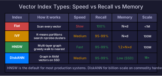
Given a query vector $q$ and a database of $N$ vectors, find the $k$ nearest neighbors:

\text{top-}k = \arg\min_{i \in \{1..N\}} \|q - v_i\|_2

Approach	Time complexity	Recall	Memory	Scale
Flat (brute-force)	$O(N \cdot d)$	100% (exact)	$O(N \cdot d)$	<1M vectors
IVF	$O(N/\text{nprobe} \cdot d)$	95-99%	$O(N \cdot d)$	1M-100M
HNSW	$O(\log N \cdot d)$	95-99%	$O(N \cdot (d + M))$	1M-100M
DiskANN	$O(\log N \cdot d)$	95-99%	$O(N \cdot d)$ on SSD	1B+

2. IVF (Inverted File Index)

Partition vectors into clusters using k-means, then search only nearby clusters:

Build: Run k-means on all vectors → C centroids
  Each vector assigned to nearest centroid's partition

Search: Find nprobe closest centroids to query
  Search only vectors in those nprobe partitions
  
  nprobe=1: fastest, lowest recall
  nprobe=C: equivalent to brute force (100% recall)

Tuning: More partitions (C) = faster search per partition, but need more nprobe for recall. Typical: C=1024-4096, nprobe=16-64.

3. HNSW (Hierarchical Navigable Small World)

A multi-layer graph where each layer is a “skip list” for the next:

Layer 2: [sparse graph — few nodes, long-range connections]
Layer 1: [medium graph — more nodes, medium connections]
Layer 0: [dense graph — all nodes, short-range connections]

Search: Start at top layer, greedily walk toward query
  → Drop to lower layer at each step for finer resolution
  → Layer 0 gives the final nearest neighbors

Pros: Very fast ( $O(\log N)$ ), high recall, no training needed. Cons: High memory (graph edges stored alongside vectors), expensive to build.

4. DiskANN

Store vectors on SSD instead of RAM — enabling billion-scale search on commodity hardware:

In-memory: compressed vector representations + graph edges
On SSD: full-precision vectors (read on demand during search)

Search: Navigate graph in memory → load candidate vectors from SSD → rerank

Key insight: The graph navigation (cheap, in memory) identifies candidates. Only the final reranking reads from SSD — minimizing I/O.

5. Choosing an Index

Your data	Best index	Why
< 100K vectors	Flat	Exact, simple, fast enough
100K - 10M	HNSW	Best recall/speed tradeoff
10M - 100M	IVF + HNSW	Combined benefits
> 100M, fits in RAM	HNSW with compression (PQ)	Compress vectors to fit
> 1B, won’t fit in RAM	DiskANN	SSD-resident, low memory

For the systems built on these indexes, see System Architecture.

Self-Check

Explain IVF partitioning and the nprobe-recall tradeoff
Explain HNSW’s multi-layer graph and why it’s O(log N)
Explain DiskANN’s split between in-memory graph and SSD vectors
Choose an index type for 50M vectors with 99% recall requirement