FlashAttention V1

FlashAttention is arguably the most impactful kernel optimization in the LLM era. By computing exact attention without materializing the $S \times S$ attention matrix, it reduces memory from $O(S^2)$ to $O(S)$ and achieves 2-4× speedup — not by reducing FLOPs, but by reducing HBM access.

---

1. The Core Insight: IO-Awareness

Standard attention is memory-bound not because of insufficient compute, but because of excessive HBM traffic. FlashAttention’s key insight: minimize reads and writes to HBM by keeping data in SRAM (shared memory).

	Naive attention	FlashAttention
Attention matrix	Materialized in HBM ($S^2$)	Never written to HBM
Softmax	Reads full row from HBM	Online softmax in SRAM
HBM traffic	$O(S^2)$	$O(S \cdot d_k)$
Memory usage	$O(S^2)$	$O(S)$
Speed	1×	2-4×

The FLOPs are identical — FlashAttention computes the exact same result. The speedup comes entirely from better IO.

---

2. Two Key Techniques

Technique 1: Tiling

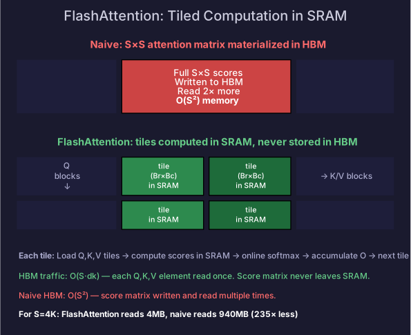
Instead of computing the full $S \times S$ matrix, process attention in tiles that fit in SRAM:

• Divide $Q$ into blocks of $B_r$ rows (e.g., 64)
• Divide $K, V$ into blocks of $B_c$ columns (e.g., 64)
• For each Q block, iterate over all K/V blocks, computing partial attention

Each tile’s intermediate results ($B_r \times B_c$ scores) live in SRAM — never touching HBM.

Technique 2: Online Softmax

The challenge: softmax needs the global maximum across the entire row, but tiling only shows part of the row at a time.

Solution: maintain running statistics $(m, \ell)$ — max and sum — and correct previous results when a new tile has a larger max:

$$m^{(new)} = \max(m^{(old)}, m^{(tile)})$$ $$\ell^{(new)} = \ell^{(old)} \cdot e^{m^{(old)} - m^{(new)}} + \ell^{(tile)} \cdot e^{m^{(tile)} - m^{(new)}}$$ $$O^{(new)} = O^{(old)} \cdot \frac{\ell^{(old)} \cdot e^{m^{(old)} - m^{(new)}}}{\ell^{(new)}} + \frac{e^{m^{(tile)} - m^{(new)}}}{\ell^{(new)}} \cdot \tilde{P}^{(tile)} V^{(tile)}$$

The output $O$ is corrected on-the-fly as each new K/V tile potentially changes the softmax normalization.

---

3. The Algorithm

Input: Q, K, V in HBM (each S × dk)
Output: O in HBM (S × dk)

For each Q block (rows i to i+Br):
    Initialize: O_i = 0, m_i = -∞, ℓ_i = 0

    For each K/V block (cols j to j+Bc):
        1. Load Q_i from HBM → SRAM       (Br × dk)
        2. Load K_j, V_j from HBM → SRAM  (Bc × dk each)

        3. Compute scores: S_ij = Q_i × K_j^T  (Br × Bc, in SRAM)
        4. Apply causal mask to S_ij

        5. Compute tile max: m_tile = rowmax(S_ij)
        6. Compute tile softmax: P_tile = exp(S_ij - m_tile)
        7. Compute tile sum: ℓ_tile = rowsum(P_tile)

        8. Update running stats:
           m_new = max(m_i, m_tile)
           ℓ_new = ℓ_i × exp(m_i - m_new) + ℓ_tile × exp(m_tile - m_new)

        9. Update output:
           O_i = O_i × (ℓ_i × exp(m_i - m_new) / ℓ_new) + (exp(m_tile - m_new) / ℓ_new) × P_tile × V_j

        10. m_i = m_new, ℓ_i = ℓ_new

    Write O_i to HBM

Key: The $B_r \times B_c$ score matrix is computed and consumed entirely in SRAM. The only HBM traffic is loading Q, K, V tiles (once each) and writing the final output O.

---

4. Memory Analysis

SRAM Usage

Per thread block:

• Q tile: $B_r \times d_k$ floats
• K tile: $B_c \times d_k$ floats
• V tile: $B_c \times d_k$ floats
• Score tile: $B_r \times B_c$ floats
• Output accumulator: $B_r \times d_k$ floats

Total: $(B_r + 2B_c) \times d_k + B_r \times B_c + B_r \times d_k$ floats

For $B_r = B_c = 128, d_k = 128$ in FP16: ~132 KB — fits in H100’s 228 KB shared memory.

HBM Traffic

$$\text{HBM reads} = S \times d_k \times 3 \text{ (Q, K, V each read once)}$$ $$\text{HBM writes} = S \times d_k \text{ (O written once)}$$ $$\text{Total} = 4 \times S \times d_k \times 2 \text{ bytes} = 8 S d_k$$

Compare naive: $\sim 14 S^2$ bytes. For $S=4096, d_k=128$: FlashAttention reads 4 MB, naive reads 940 MB. 235× less HBM traffic.

---

5. The Backward Pass

FlashAttention doesn’t store the $S \times S$ attention matrix — so how does the backward pass access it?

Recomputation: During backward, FlashAttention recomputes the attention scores from Q, K, V (still in HBM). This costs extra FLOPs but saves the $O(S^2)$ memory that would be needed to store attention weights for backward.

The tradeoff: ~25-33% more FLOPs in backward, but $O(S)$ memory instead of $O(S^2)$. For long sequences, this is overwhelmingly worth it.

---

6. Practical Impact

Metric	Naive	FlashAttention V1
Memory	$O(S^2)$	$O(S)$
HBM traffic	$O(S^2 d_k)$	$O(S d_k)$
Speed (S=2K)	1×	~2×
Speed (S=16K)	OOM	~3-4× (vs what would be possible)
Max sequence length (H100)	~32K	Unlimited (bounded by KV cache, not attention matrix)

FlashAttention didn’t just make attention faster — it made long-context LLMs possible.

---

Self-Check

• Explain the IO-awareness principle — why reducing HBM traffic is more important than reducing FLOPs
• Explain the two key techniques: tiling and online softmax
• Trace through one iteration of the algorithm for a single Q block and K/V block
• Calculate SRAM usage for given Br, Bc, dk and verify it fits in shared memory
• Compare HBM traffic: naive vs FlashAttention for S=4096
• Explain why the backward pass recomputes attention scores instead of storing them

---

References

• FlashAttention: Fast and Memory-Efficient Exact Attention (Dao et al., 2022)
• Online Normalizer Calculation for Softmax (Milakov & Gimelshein, 2018)
• Self-Attention Does Not Need O(n²) Memory (Rabe & Staats, 2021)