Back-of-Envelope Estimation

The ability to estimate — before running a single experiment — whether something will work, how long it will take, and what will be the bottleneck is the single most valuable skill in AI infrastructure. This chapter is a collection of worked examples that build that intuition.

---

1. The Three Estimates

For any AI workload, you need three numbers:

1. Memory: will the model + data fit in GPU memory?
2. Compute: how long will it take?
3. Bottleneck: is it compute-bound or memory-bound?

Getting these right (within 2×) before writing any code saves weeks of wasted GPU time.

---

2. Memory Estimation

Model Weight Memory

$$\text{Weight memory} = N_{\text{params}} \times \text{bytes per param}$$

Precision	Bytes/param	7B model	70B model
FP32	4	28 GB	280 GB
BF16 / FP16	2	14 GB	140 GB
FP8	1	7 GB	70 GB
INT4	0.5	3.5 GB	35 GB

Training Memory (Adam + BF16 Mixed Precision)

Component	Bytes/param	7B model
BF16 parameters	2	14 GB
FP32 master weights	4	28 GB
FP32 gradients	4	28 GB
Adam m (FP32)	4	28 GB
Adam v (FP32)	4	28 GB
Total fixed	18	126 GB

Plus activation memory (depends on batch size and sequence length):

$$\text{Activation per layer} \approx 2 \times B \times S \times d \times \text{bytes} + B \times N_h \times S^2 \times \text{bytes}$$

For 7B, $B=1, S=2048$: ~0.5 GB per layer × 32 layers = ~16 GB. With gradient checkpointing, this drops to ~$\sqrt{32} \times 0.5$ GB ≈ 3 GB.

Total training memory (7B): ~126 GB fixed + 3–16 GB activations = ~130–142 GB → needs 2× H100 (80GB each) minimum with ZeRO.

KV Cache Memory (Inference)

$$\text{KV cache per token} = 2 \times L \times N_{kv} \times d_k \times \text{bytes}$$

Model	Config	Per token (FP16)	4K context	128K context
LLaMA-2-7B (MHA)	$L=32, N_{kv}=32, d_k=128$	512 KB	2 GB	64 GB
LLaMA-2-70B (GQA-8)	$L=80, N_{kv}=8, d_k=128$	320 KB	1.3 GB	40 GB
Mistral-7B (GQA-8)	$L=32, N_{kv}=8, d_k=128$	128 KB	512 MB	16 GB

Inference total memory = model weights + KV cache for all concurrent requests:

For 7B FP16 serving 32 concurrent requests at 4K context:

• Weights: 14 GB
• KV cache: 32 × 2 GB = 64 GB
• Total: 78 GB → barely fits one H100

This is why KV cache is the primary memory constraint for inference, and why GQA/quantization matter so much.

---

3. Compute Estimation

Training FLOPs

$$C \approx 6ND$$

Where $N$ = parameters, $D$ = training tokens. The 6× accounts for forward (2 FLOPs per param per token) + backward (4 FLOPs).

Training Time

$$T = \frac{C}{\text{GPU count} \times \text{FLOPS/GPU} \times \text{MFU}}$$

Worked example: Train a 7B model on 2T tokens with 64 H100s at 40% MFU:

$$C = 6 \times 7 \times 10^9 \times 2 \times 10^{12} = 8.4 \times 10^{22} \text{ FLOPs}$$ $$T = \frac{8.4 \times 10^{22}}{64 \times 989 \times 10^{12} \times 0.4} = \frac{8.4 \times 10^{22}}{2.53 \times 10^{16}} = 3.32 \times 10^6 \text{ s} \approx \textbf{38 days}$$

Inference Latency

Prefill latency (compute-bound):

$$T_{\text{prefill}} \approx \frac{2 \times N \times S}{\text{TFLOPS} \times 10^{12}}$$

For 7B, S=2048 on H100 (989 TFLOPS FP16) — this is the theoretical minimum at 100% utilization; multiply by 1/MFU (typically 2-3×) for realistic estimates:

$$T_{\text{prefill}} = \frac{2 \times 7 \times 10^9 \times 2048}{989 \times 10^{12}} = \frac{2.87 \times 10^{13}}{9.89 \times 10^{14}} \approx 29 \text{ ms}$$

Decode latency per token (memory-BW-bound):

$$T_{\text{decode}} \approx \frac{2 \times N \times \text{bytes/param}}{\text{BW (bytes/s)}}$$

For 7B FP16 on H100 (3,350 GB/s):

$$T_{\text{decode}} = \frac{2 \times 7 \times 10^9 \times 2}{3.35 \times 10^{12}} = \frac{2.8 \times 10^{10}}{3.35 \times 10^{12}} \approx 8.4 \text{ ms/token}$$

This gives ~119 tokens/second for a single request — the theoretical maximum for 7B FP16 on H100. Real-world is lower due to attention KV cache reads and overhead.

Batching changes the equation: With 32 concurrent requests, you read the weights once and process 32 tokens simultaneously. Theoretical throughput: $32 \times 119 \approx 3,800$ tokens/second. This is why batching is the most important inference optimization — it amortizes the weight-read cost across many requests.

Why decode reads the full model per token: Each generated token requires a forward pass through all layers. With batch size 1, the weight matrices dominate memory reads — the same 14 GB of weights are read from HBM for every single token.

---

4. Bottleneck Analysis: The Roofline

Arithmetic Intensity

$$\text{AI} = \frac{\text{FLOPs}}{\text{Bytes accessed}}$$

Compare to the GPU’s ops:byte ratio:

$$\text{Ridge point} = \frac{\text{Peak FLOPS}}{\text{Peak bandwidth}} = \frac{989 \times 10^{12}}{3.35 \times 10^{12}} = 295 \text{ FLOPs/byte (H100 FP16)}$$

• AI > 295 → compute-bound (GPU math units are the limit)
• AI < 295 → memory-BW-bound (data transfer is the limit)

Common Operations

Operation	Typical AI	Bound
Large GEMM (training, prefill)	500–2000	Compute ✅
Small GEMM (decode, M=1)	~1	Memory-BW ❌
FlashAttention (fused)	50–200	Depends on sequence length
LayerNorm	~5	Memory-BW ❌
Softmax	~2	Memory-BW ❌
Element-wise (activation, residual)	~1	Memory-BW ❌

Key insight: Most operations in an LLM are memory-bound. Only large matrix multiplications (training batch GEMMs, long-context prefill) are compute-bound. This is why:

• Kernel fusion (combining multiple memory-bound ops into one kernel) is critical
• Batching (combining M=1 decode requests into M=B) is essential for inference throughput
• FlashAttention (reducing memory access by computing in SRAM tiles) provides huge speedups

---

5. Putting It All Together: Worked Examples

Example 1: Can I fine-tune LLaMA-2-70B on one 8×H100 node?

• Weight memory (BF16): $70B \times 2 = 140$ GB
• With LoRA (only adapters in optimizer): ~140 GB weights + ~2 GB optimizer ≈ 142 GB
• 8 × 80 GB = 640 GB available with ZeRO-3
• Activations (B=1, S=4096): ~80 GB without checkpointing, ~15 GB with checkpointing
• Answer: Yes, with LoRA + gradient checkpointing + ZeRO-3. Total ~157 GB across 8 GPUs (~20 GB each).

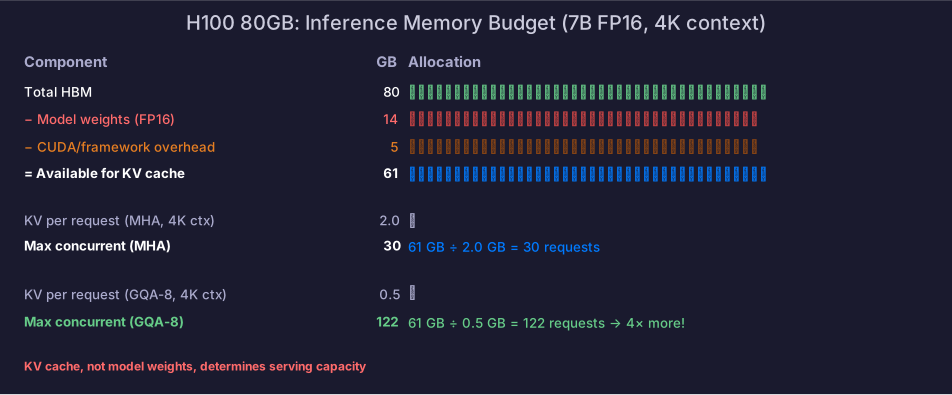
Example 2: How many concurrent 7B requests can one H100 serve?

• Model weights (FP8): 7 GB
• Available for KV cache: 80 - 7 - 5 (overhead) = 68 GB
• KV cache per request at 4K context (MHA, FP16): 2 GB
• Max concurrent requests: 68 / 2 = 34 requests
• With GQA-8 (128 KB/token): 68 GB / 0.5 GB per 4K req = 136 requests

Example 3: Training time for 405B on 15T tokens

• FLOPs: $6 \times 405 \times 10^9 \times 15 \times 10^{12} = 3.6 \times 10^{25}$
• With 16,000 H100s at 45% MFU:
• $T = \frac{3.6 \times 10^{25}}{16000 \times 989 \times 10^{12} \times 0.45} = \frac{3.6 \times 10^{25}}{7.12 \times 10^{18}} = 5.06 \times 10^6 \text{ s} \approx$ 58 days
• This matches Meta’s reported training time for LLaMA 3.1 405B.

Memory check: $405B \times 18 \text{ bytes/param} = 7.3$ TB for weights+optimizer. At 80 GB per H100, that’s a minimum of 92 GPUs just to hold the model state (before activations). With ZeRO-3 across 16,000 GPUs, each GPU holds ~0.46 GB of sharded state — memory is not the constraint at this scale; communication is.

---

5.5. Validating Your Estimates

Estimates are only useful if you check them against reality. The gap between estimate and measurement reveals hidden costs.

How to Measure

# Decode throughput (single request)
python -c "
import torch, time
model = load_model('llama-7b').cuda().half()
tokens = torch.randint(0, 32000, (1, 1)).cuda()
kv_cache = prefill(model, prompt)

torch.cuda.synchronize()
start = time.perf_counter()
for _ in range(100):
    tokens, kv_cache = decode_one(model, tokens, kv_cache)
torch.cuda.synchronize()
elapsed = time.perf_counter() - start
print(f'{100/elapsed:.1f} tokens/sec')
"

# GPU utilization during decode
nvidia-smi dmon -s u -d 1   # SM utilization, memory BW utilization

# Memory breakdown
print(torch.cuda.memory_summary())

What to Compare

Metric	Estimate	Typical measured	Gap cause
Decode tok/s (7B, FP16, B=1)	119	60–90	Kernel launch overhead, KV cache reads, attention compute
Prefill latency (7B, S=2048)	29 ms	40–60 ms	MFU < 100%, memory allocation, framework overhead
Training MFU	100% (theoretical)	35–55%	Communication, pipeline bubbles, data loading stalls
KV cache memory	Formula exact	+10-20%	Memory fragmentation, PyTorch allocator overhead

Diagnostic Checklist: When Estimates Diverge

If measured performance is much worse than estimated:

Symptom	Likely cause	How to confirm
Decode 2× slower than estimate	KV cache attention reads not accounted for	Profile: check if attention kernel time dominates
Prefill 3× slower than estimate	Low MFU (small batch, framework overhead)	Check nvidia-smi: SM utilization should be >80% for prefill
Training 2× slower than estimate	Communication overhead (gradient sync)	Profile: check AllReduce time vs compute time
Memory 30% higher than estimate	Activation memory, fragmentation, framework buffers	torch.cuda.memory_summary() shows allocated vs reserved
Memory exactly matches but OOM anyway	Peak memory spike during allocation	Set PYTORCH_CUDA_ALLOC_CONF=expandable_segments:True

The gap between estimate and reality IS the optimization opportunity. If your estimate says 119 tok/s but you measure 70 tok/s, the 49 tok/s gap is quantified waste — now you know exactly how much headroom exists.

Example 4: Prefill latency for 70B on 8×H100 (TP=8)

With tensor parallelism, each GPU handles 1/8 of the model:

• Per-GPU weight reads: $140 \text{ GB} / 8 = 17.5$ GB
• FLOPs per GPU: $2 \times 70B \times 2048 / 8 = 3.6 \times 10^{13}$
• Compute time per GPU: $3.6 \times 10^{13} / (989 \times 10^{12}) \approx 36$ ms
• NVLink communication (AllReduce per layer): ~32 AllReduces × ~0.1 ms each ≈ 3 ms
• Estimated total: ~39 ms prefill (in practice: 50–80 ms due to MFU < 100%)

Key insight: with TP=8, prefill is still compute-bound — NVLink overhead is <10% of total time. This is why tensor parallelism works well on NVLink-connected GPUs.

---

6. Common Estimation Mistakes

Mistake	Reality
“Model fits in memory = can serve”	Forgot KV cache — the real constraint at serving time
“Doubled GPUs = halved time”	Communication overhead reduces scaling efficiency to 70–90%
“Peak TFLOPS = real performance”	Real MFU is 30–55%; use effective TFLOPS
“FP16 model = 2 bytes/param”	Forgot optimizer states in training (18 bytes/param with Adam)
“Faster than before = well optimized”	Without roofline analysis, you might be at 10% of hardware ceiling
“Scaling law optimal = production optimal”	Inference cost dominates — over-training small models is often better

---

Self-Check

• Estimate memory for a 13B model in training (Adam + BF16) vs inference (FP16)
• Calculate KV cache size for a given model config and context length
• Estimate training time given model size, token count, GPU count, and MFU
• Calculate theoretical decode latency from model size and HBM bandwidth
• Determine if a given operation is compute-bound or memory-bound using arithmetic intensity
• Estimate max concurrent requests for a given GPU and model

---

References

• LLM Parameter Counting (Kipply)
• Efficiently Scaling Transformer Inference (Pope et al., 2022)
• Roofline Model (Williams et al., 2009)
• NVIDIA H100 Datasheet