Linear Algebra for AI Infrastructure

AI infrastructure doesn’t require proving theorems daily, but it requires that when you see a formula, you can immediately answer three engineering questions: what shape are the tensors, how much compute and memory does it cost, and what can go wrong numerically?

This chapter builds that intuition for linear algebra — the mathematical foundation underlying every matrix multiply, every attention computation, and every GPU kernel optimization.

---

1. Three Questions for Every Formula

Take the language model output projection as an example:

$$\mathbf{Y} = \mathbf{X}\mathbf{W}, \qquad \mathbf{X} \in \mathbb{R}^{(BS) \times H},\quad \mathbf{W} \in \mathbb{R}^{H \times V}$$

Question 1 — Shape: Do the inner dimensions match? $H = H$ ✓. Output is $(BS) \times V$.

Question 2 — Cost: Each output element requires $H$ multiply-adds. Total: $2BSHV$ FLOPs (counting one multiply + one add as 2 ops).

Question 3 — Risk: Large weights → large logits → numerical instability in softmax. Need to consider dtype, memory layout, tiling strategy, and numerical stability.

These three questions apply to every operation in the AI infrastructure stack.

Notation

Symbol	Meaning
$x$	Scalar
$\mathbf{x}$	Vector
$\mathbf{X}$	Matrix or higher-order tensor
$B, S, H, V$	Batch size, sequence length, hidden size, vocabulary size
$N_h, D_h = H/N_h$	Number of attention heads, dimension per head
$\odot$	Element-wise multiplication

---

2. Scalars, Vectors, Matrices, and Tensors

• Scalar: a single number — e.g., learning rate $\eta = 10^{-4}$
• Vector: 1D array — e.g., a token’s hidden state $\mathbf{x} \in \mathbb{R}^{H}$
• Matrix: 2D array — e.g., linear layer weights $\mathbf{W} \in \mathbb{R}^{H \times 4H}$
• Tensor: N-dimensional array — e.g., a batch of sequences $\mathbf{X} \in \mathbb{R}^{B \times S \times H}$

In engineering, a “tensor” carries more than just shape:

data pointer + shape + stride + dtype + device + layout

Two tensors with the same shape may have different memory layouts. Two tensors with the same values may have different dtypes and different numerical error characteristics.

Shape, Indexing, and Stride

A $(2, 3)$ row-major matrix:

$$\mathbf{X} = \begin{bmatrix} 1 & 2 & 3 \\ 4 & 5 & 6 \end{bmatrix}$$

Stored contiguously as [1, 2, 3, 4, 5, 6] with stride $(3, 1)$. Element $X_{ij}$ is at offset $3i + j$.

Transpose $\mathbf{X}^\top$ has shape $(3, 2)$ and stride $(1, 3)$ — no data copy needed. But scanning along the last dimension is no longer contiguous in memory — this matters for GPU coalescing.

When you see view, reshape, transpose, or contiguous in PyTorch, always think about both the logical dimensions and the physical memory layout.

Broadcasting

Element-wise operations require matching shapes. Broadcasting allows dimensions of size 1 (or missing) to be logically expanded:

$$\mathbf{X} \in \mathbb{R}^{B \times S \times H}, \quad \mathbf{b} \in \mathbb{R}^{H} \quad \Rightarrow \quad \mathbf{X} + \mathbf{b} \in \mathbb{R}^{B \times S \times H}$$

The bias $\mathbf{b}$ is reused across batch and sequence dimensions without copying.

Rules (align from the trailing dimension):

1. Both sizes are equal, or
2. One of them is 1, or
3. One side has no dimension there

Danger: Wrong shapes may “accidentally broadcast” — code runs without error but computes the wrong thing. Always verify shapes explicitly.

Norms

Norms measure the “size” of a vector or matrix:

• L1 norm: $\|\mathbf{x}\|_1 = \sum_i |x_i|$ — used in sparse regularization
• L2 norm: $\|\mathbf{x}\|_2 = \sqrt{\sum_i x_i^2}$ — Euclidean distance, used in gradient clipping
• Frobenius norm: $\|\mathbf{X}\|_F = \sqrt{\sum_{ij} X_{ij}^2}$ — the matrix equivalent of L2
• Max norm: $\|\mathbf{x}\|_\infty = \max_i |x_i|$

In AI infra, norms appear everywhere:

• Gradient clipping: if $\|\nabla\|_2 > \text{threshold}$, scale down
• Weight decay: adds $\lambda \|\mathbf{W}\|_2^2$ to loss, penalizing large weights
• Layer normalization: divides by $\sqrt{\sum x_i^2}$ (related to RMS norm)

---

3. Dot Product and Matrix Multiplication

Dot Product

$$\mathbf{x}^\top \mathbf{y} = \sum_{i=1}^{n} x_i y_i$$

Two intuitions:

• Weighted sum: $\mathbf{x}$ is weights, $\mathbf{y}$ is values
• Similarity: normalized dot product = cosine similarity. Larger means more aligned.

This is the core operation inside attention: query-key dot products measure how much each key “matches” the query.

Matrix Multiplication

Matrix multiply is a batch of dot products:

$$C_{ij} = \sum_{k=1}^{K} A_{ik} B_{kj}$$

For $\mathbf{A} \in \mathbb{R}^{M \times K}$ and $\mathbf{B} \in \mathbb{R}^{K \times N}$:

• Output shape: $(M, N)$
• FLOPs: $2MKN$ (each of $MN$ elements requires $K$ multiply-adds)
• Memory reads: $MK + KN$ elements
• Memory writes: $MN$ elements

Batched Matrix Multiplication

In transformers, matmuls are batched over multiple heads and batch dimensions:

$$\mathbf{C}[b, h] = \mathbf{A}[b, h] \times \mathbf{B}[b, h]$$

Shape: $(B, N_h, S, D_h) \times (B, N_h, D_h, S) \rightarrow (B, N_h, S, S)$

This is exactly the attention score computation: $\mathbf{Q}\mathbf{K}^\top$.

---

4. GEMM Tiling: Why It Matters for GPU Kernels

General Matrix Multiply (GEMM) is the most performance-critical operation in deep learning. Understanding tiling explains why GPU kernels are fast — and when they’re not.

Block Decomposition

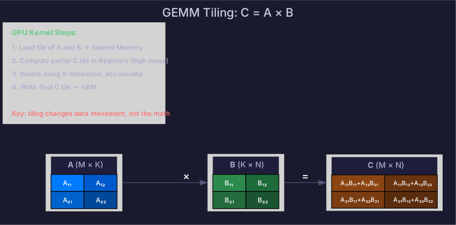
Split matrices into tiles along $M$, $N$, and the reduction dimension $K$:

$$\mathbf{C}_{11} = \mathbf{A}_{11}\mathbf{B}_{11} + \mathbf{A}_{12}\mathbf{B}_{21}$$

Each output tile accumulates partial products along $K$. The GPU kernel:

1. Loads a tile of $\mathbf{A}$ and $\mathbf{B}$ into shared memory
2. Computes partial output using registers (high reuse)
3. Iterates along $K$, accumulating
4. Writes the final output tile back to HBM

This changes data movement order, not the mathematical result.

Arithmetic Intensity of GEMM

For a $(M, K) \times (K, N)$ multiply:

$$\text{FLOPs} = 2MKN, \qquad \text{Bytes} = 2(MK + KN + MN) \text{ (FP16)}$$ $$\text{Arithmetic Intensity} = \frac{2MKN}{2(MK + KN + MN)}$$

For square matrices ($M = N = K = n$):

$$\text{AI} \approx \frac{2n^3}{6n^2} = \frac{n}{3}$$

A 4096×4096 GEMM has AI ≈ 1365 — well above the H100’s ops:byte ratio of 295. Large GEMMs are compute-bound. But small GEMMs (like per-token decode with $M = 1$) have AI ≈ 1 — severely memory-bound.

This is why LLM decode is slow: each token generates a GEMM with $M = 1$, which can never saturate GPU compute.

Tile Size Tradeoffs

Larger tiles	Smaller tiles
✅ Higher data reuse → higher arithmetic intensity	✅ Less shared memory per tile → more tiles per SM
✅ Fewer trips to HBM	✅ Better occupancy
❌ More shared memory → lower occupancy	❌ More HBM trips
❌ Tail blocks waste compute if dimensions aren’t divisible	✅ Less waste on irregular shapes

Optimal tile size depends on the GPU’s shared memory capacity, register count, and the specific matrix dimensions. This is what autotuners like cuBLAS and Triton’s compiler optimize.

---

5. SVD and Low-Rank Approximation (LoRA Connection)

Any matrix $\mathbf{W} \in \mathbb{R}^{m \times n}$ can be decomposed:

$$\mathbf{W} = \mathbf{U} \boldsymbol{\Sigma} \mathbf{V}^\top$$

Where $\mathbf{U}$ and $\mathbf{V}$ are orthogonal matrices and $\boldsymbol{\Sigma}$ is diagonal with singular values $\sigma_1 \geq \sigma_2 \geq \cdots$.

Keeping only the top $r$ singular values gives the best rank-$r$ approximation:

$$\mathbf{W} \approx \mathbf{U}_r \boldsymbol{\Sigma}_r \mathbf{V}_r^\top$$

Why this matters for AI infra: LoRA (Low-Rank Adaptation) freezes the pretrained weight $\mathbf{W}_0$ and adds a low-rank update:

$$\mathbf{W} = \mathbf{W}_0 + \mathbf{B}\mathbf{A}, \qquad \mathbf{B} \in \mathbb{R}^{m \times r}, \quad \mathbf{A} \in \mathbb{R}^{r \times n}$$

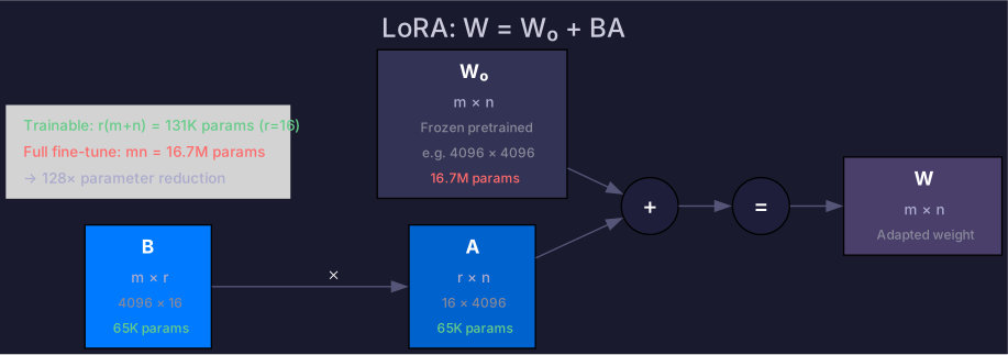
Instead of fine-tuning $mn$ parameters, you train only $r(m + n)$ parameters. With $r = 16$ and $m = n = 4096$, that’s a 128× parameter reduction.

This directly impacts infrastructure: LoRA adapters are small enough to hot-swap in serving, store hundreds per GPU, and fine-tune on a single consumer GPU.

---

Self-Check

• Given two tensor shapes, determine if matrix multiplication is valid and predict the output shape
• Calculate the FLOPs for a given matrix multiplication
• Explain why large GEMMs are compute-bound but small GEMMs ($M=1$) are memory-bound
• Explain stride and why transpose doesn’t copy data
• Identify broadcasting bugs: given two shapes, predict if they broadcast and what the result shape is
• Explain why LoRA reduces trainable parameters and its infrastructure implications
• Calculate arithmetic intensity for a GEMM and compare to the GPU’s ops:byte ratio

---

References

• The Matrix Cookbook — comprehensive matrix identity reference
• 3Blue1Brown — Essence of Linear Algebra — visual intuition
• LoRA: Low-Rank Adaptation of Large Language Models
• NVIDIA cuBLAS Documentation