From Transformer to Autoregressive LLM

A Transformer is trained to predict the next token. Turning that into a conversational AI that generates paragraphs of text requires an autoregressive loop — and understanding this loop is the foundation for all inference optimization.

1. Language Modeling: Predicting the Next Token

A language model factorizes the probability of a sequence using the chain rule:

P(x_1, x_2, \ldots, x_T) = \prod_{t=1}^{T} P(x_t \mid x_1, \ldots, x_{t-1})

At each position, the model outputs a probability distribution over the entire vocabulary:

\text{logits}_t = \text{LM\_Head}(\text{TransformerBlocks}(\text{Embed}(x_1, \ldots, x_t)))

P(x_{t+1} \mid x_1, \ldots, x_t) = \text{softmax}(\text{logits}_t / T)

The next token is sampled from this distribution. Then the sampled token is appended to the input and the process repeats.

2. The Generation Loop

def generate(model, prompt_tokens, max_new_tokens, temperature=1.0):
    tokens = prompt_tokens  # list of token IDs

    for _ in range(max_new_tokens):
        # Forward pass: all tokens → logits for next position
        logits = model(tokens)[:, -1, :]   # take last position's logits

        # Sample next token
        probs = softmax(logits / temperature)
        next_token = sample(probs)

        tokens.append(next_token)

        if next_token == EOS_TOKEN:
            break

    return tokens

This is inherently sequential — each token depends on all previous tokens. You cannot parallelize across the output sequence. This is the fundamental reason LLM inference is hard.

3. Prefill and Decode: Two Phases

Every generation request has two distinct phases with completely different compute characteristics:

Prefill vs Decode

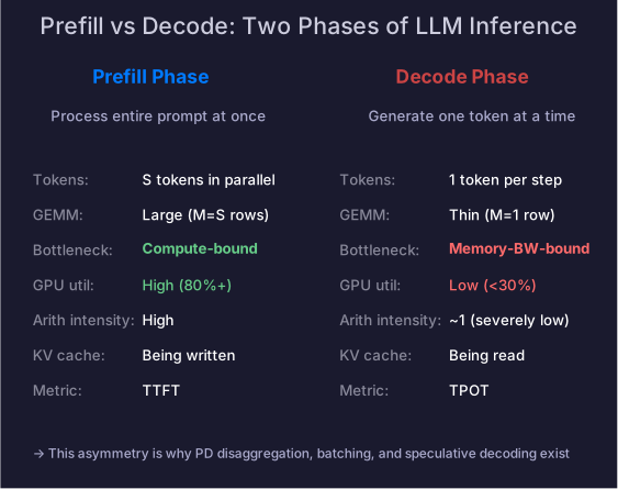
Prefill Phase

Process the entire input prompt in parallel:

Input: [tok1, tok2, tok3, ..., tokN]  (N tokens)
  → One forward pass
  → Compute KV cache for all N tokens
  → Output: logits for position N+1

Compute pattern: Large matrix multiplications with $S = N$
Bottleneck: Compute-bound (GPU is busy doing math)
Metric: TTFT (Time to First Token)

Decode Phase

Generate tokens one at a time:

Step 1: [tok1...tokN, tokN+1]  → logits → sample tokN+2
Step 2: [tok1...tokN+1, tokN+2] → logits → sample tokN+3
  ...each step adds one token

But with KV cache, each decode step only processes the new token:

Step 1: Process ONLY tokN+1 (reuse KV cache for tok1...tokN)
Step 2: Process ONLY tokN+2 (reuse KV cache for tok1...tokN+1)

Compute pattern: Tiny matrix multiplications with $S = 1$
Bottleneck: Memory-bandwidth-bound (GPU is waiting for data)
Metric: TPOT (Time Per Output Token)

Why This Matters for Infrastructure

Property	Prefill	Decode
Tokens processed	All at once	One at a time
Compute pattern	Large GEMM ( $S$ rows)	Thin GEMM ( $M = 1$ )
Bottleneck	Compute-bound	Memory-bandwidth-bound
GPU utilization	High (80%+)	Low (often <30%)
Arithmetic intensity	High	~1 (severely memory-bound)
KV cache	Being written	Being read

This is why:

Prefill-decode disaggregation uses separate GPU pools for each phase
Batching is critical for decode — aggregate many $M=1$ GEMMs into one $M=B$ GEMM
KV cache is the dominant memory consumer at serving time
Speculative decoding tries to parallelize the sequential decode

4. KV Cache

KV Cache Growth

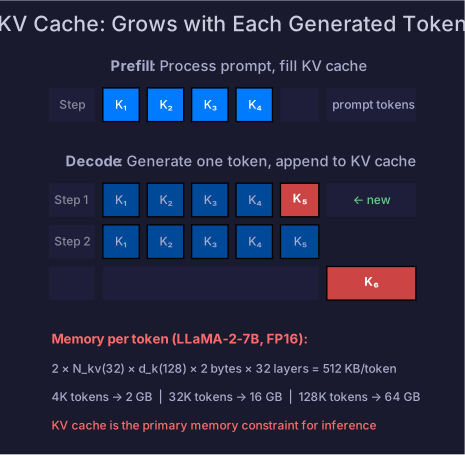
Without KV cache, generating token $t+1$ requires reprocessing all $t$ previous tokens — $O(t^2)$ total work for a sequence.

With KV cache:

Prefill: compute and store K, V for all input tokens
Each decode step: compute K, V only for the new token, append to cache, use full cache for attention

Cache size per token per layer (FP16):

2 \times N_{kv} \times d_k \times 2 \text{ bytes}

For LLaMA-2-7B ( $N_{kv}=32, d_k=128$ , 32 layers):

Per token: $32 \times 2 \times 32 \times 128 \times 2 = 512$ KB
For 4K tokens: 2 GB
For 128K tokens: 64 GB

KV cache is the primary memory constraint for inference — it determines how many concurrent requests a GPU can serve. This is why GQA, MLA, and KV cache quantization exist.

5. Sampling Strategies

The model outputs logits — how we convert them to token selections affects output quality:

Greedy Decoding

Always pick the highest-probability token: $\text{argmax}(P)$

Deterministic, fast
Often repetitive and boring
Used for benchmarking, not production

Temperature Scaling

P(x) = \text{softmax}(\text{logits} / T)

$T < 1$ : sharper distribution (more deterministic)
$T > 1$ : flatter distribution (more random/creative)
$T \to 0$ : equivalent to greedy

Top-k Sampling

Keep only the $k$ highest-probability tokens, zero out the rest, renormalize:

topk_logits, topk_indices = logits.topk(k)
probs = softmax(topk_logits)
next_token = topk_indices[sample(probs)]

Top-p (Nucleus) Sampling

Keep the smallest set of tokens whose cumulative probability $\geq p$ :

sorted_probs, sorted_indices = probs.sort(descending=True)
cumsum = sorted_probs.cumsum(dim=-1)
mask = cumsum - sorted_probs > p  # remove tokens beyond threshold
sorted_probs[mask] = 0
sorted_probs /= sorted_probs.sum()  # renormalize

Adaptive: for confident predictions (one token has 90% probability), top-p effectively picks ~1 token. For uncertain predictions, it considers many tokens.

Infrastructure Note

Sampling parameters (temperature, top-k, top-p) are per-request serving parameters — different users may want different settings. The serving infrastructure must support per-request configuration without reloading the model.

6. Multi-Token Prediction (MTP)

Standard autoregressive LLMs predict one token at a time. Multi-token prediction adds auxiliary prediction heads that forecast multiple future tokens simultaneously:

\text{Head}_k(\mathbf{h}_t) \to P(x_{t+k}) \qquad k = 1, 2, \ldots, K

During training: all K heads are trained jointly, providing richer gradient signal (each position gets feedback from K predictions, not just 1). This improves sample efficiency.

During inference: the auxiliary heads enable speculative verification — the model proposes K tokens at once, then verifies them in a single forward pass. If predictions are correct, K tokens are accepted at the cost of ~1 forward pass. This is architecturally native speculative decoding (no separate draft model needed).

DeepSeek-V3 uses MTP as a core architecture feature — the auxiliary heads are trained alongside the main model and used for both better training and faster inference.

7. Beam Search vs Sampling

Beam search maintains the top-B most probable partial sequences and expands them in parallel:

Beam 1: "The cat" → "The cat sat" (score: -2.3)
Beam 2: "The dog" → "The dog ran" (score: -2.5)
Beam 3: "The cat" → "The cat ran" (score: -2.7)
→ Keep top-B, discard rest, continue

Used in translation and structured generation where quality matters more than diversity
Produces more “correct” but less creative output than sampling
Largely replaced by sampling for open-ended LLM generation — beam search tends to produce generic, repetitive text

Repetition Penalty

A common serving parameter: penalize tokens that have already appeared:

\text{logits}[t] = \text{logits}[t] / \text{penalty} \quad \text{if token } t \text{ appeared before}

With penalty > 1.0, repeated tokens become less likely. Typical value: 1.1–1.3.

8. Streaming

In production, tokens are delivered to the client as they’re generated — not after the full response:

Server-Sent Events (SSE):

data: {"token": "The"}
data: {"token": " capital"}
data: {"token": " of"}
data: {"token": " France"}
data: {"token": " is"}
data: {"token": " Paris"}
data: {"token": "."}
data: [DONE]

Infrastructure requirements:

Long-lived HTTP connections (not request-response)
Backpressure handling: if the client can’t consume tokens fast enough, the server must buffer or slow down
Token-level latency matters: users perceive the stream speed, not just total time
Connection management at scale: thousands of concurrent streaming connections per GPU