Calculus & Probability for AI Infrastructure

If linear algebra is the language of the forward pass, then calculus and probability are the language of training. This chapter covers the math that directly impacts AI infrastructure: stable softmax computation, cross-entropy loss, backpropagation mechanics, gradient stability, and the numerical precision tradeoffs behind mixed-precision training.

1. Probability Essentials

Random Variables and Distributions

A language model outputs a probability distribution over the vocabulary at each step. The key concepts:

Discrete distribution: $P(X = v_i) = p_i$ where $\sum_i p_i = 1$
Expectation: $\mathbb{E}[X] = \sum_i x_i p_i$ — the probability-weighted average
Variance: $\text{Var}(X) = \mathbb{E}[(X - \mu)^2]$ — spread around the mean
Mini-batch estimates: sample mean $\bar{x} = \frac{1}{n}\sum x_i$ approximates $\mathbb{E}[X]$

Maximum Likelihood and Negative Log-Likelihood

Given training data, maximum likelihood estimation (MLE) finds parameters that maximize $\prod_i P(x_i \mid \theta)$ . Taking the log turns the product into a sum, and negating turns maximization into minimization:

\mathcal{L} = -\sum_i \log P(x_i \mid \theta)

This is negative log-likelihood (NLL) — the loss function used for language model training. Minimizing NLL = maximizing the probability of the training data.

2. Softmax: From Logits to Probabilities

Logits Are Not Probabilities

The model’s final layer outputs $V$ arbitrary real numbers (logits):

\mathbf{z} = (z_1, z_2, \ldots, z_V)

Softmax converts them to a valid probability distribution:

p_i = \frac{e^{z_i}}{\sum_{j=1}^{V} e^{z_j}}

Clearly $p_i > 0$ and $\sum_i p_i = 1$ . Softmax is invariant to uniform shifts: $\text{softmax}(\mathbf{z} + c) = \text{softmax}(\mathbf{z})$ . This property is the basis of the stable implementation.

Numerically Stable Softmax

Computing $e^{1000}$ directly overflows. The fix: subtract the maximum first.

m = \max_j z_j, \qquad p_i = \frac{e^{z_i - m}}{\sum_j e^{z_j - m}}

The largest exponent input becomes 0, so the largest exponential value is 1. All others are ≤ 1.

def stable_softmax(x):
    m = max(x)
    exps = [exp(v - m) for v in x]
    total = sum(exps)
    return [v / total for v in exps]

If you need $\log(\text{softmax})$ afterward, compute log_softmax directly — don’t softmax first then log, because softmax may underflow to 0, making $\log(0) = -\infty$ .

LogSumExp

\text{LSE}(\mathbf{z}) = \log \sum_j e^{z_j} = m + \log \sum_j e^{z_j - m}

Then: $\log \text{softmax}(\mathbf{z})_i = z_i - \text{LSE}(\mathbf{z})$

Why this matters for infrastructure: Cross-entropy implementations fuse log_softmax + NLLLoss into a single kernel. This reduces intermediate tensors (less memory), reduces HBM access (fewer kernel launches), and avoids the numerical instability of “softmax then log.”

Temperature

p_i = \frac{e^{z_i / T}}{\sum_j e^{z_j / T}}

$T \to 0$ : distribution becomes one-hot (greedy)
$T = 1$ : standard softmax
$T > 1$ : flatter distribution (more random)

Temperature is a serving parameter — the same model weights produce different behavior. Infrastructure must support per-request temperature.

Cross-Entropy Loss

Given true distribution $\mathbf{y}$ (one-hot: $y_c = 1$ for the correct class) and predicted $\hat{\mathbf{y}}$ :

H(\mathbf{y}, \hat{\mathbf{y}}) = -\sum_i y_i \log \hat{y}_i = -\log \hat{y}_c

For language models, this is computed per token and averaged over the sequence.

Perplexity

\text{PPL} = e^{H} = e^{-\frac{1}{N}\sum_{i=1}^{N} \log P(x_i)}

Perplexity = “how many choices the model is confused between.” Lower is better. PPL of 10 means the model is, on average, choosing between 10 equally likely next tokens.

Perplexity is the standard evaluation metric reported for language models and is directly derived from cross-entropy loss.

KL Divergence

KL divergence measures how one distribution $P$ differs from another $Q$ :

D_{KL}(P \| Q) = \sum_i P(i) \log \frac{P(i)}{Q(i)}

Properties: $D_{KL} \geq 0$ , equals 0 only when $P = Q$ , and is not symmetric ( $D_{KL}(P\|Q) \neq D_{KL}(Q\|P)$ ).

Where it appears in AI infra:

RLHF: KL penalty prevents the policy from diverging too far from the reference model: $R_{\text{total}} = R_{\text{reward}} - \beta \cdot D_{KL}(\pi \| \pi_{\text{ref}})$
Knowledge distillation: student minimizes $D_{KL}(P_{\text{teacher}} \| P_{\text{student}})$
Evaluating distribution shift in production monitoring

Top-k and Top-p Sampling

Sampling strategies for generation — these are serving parameters, not training parameters:

Top-k: Keep only the $k$ highest-probability tokens, redistribute mass among them.

Top-p (nucleus): Keep the smallest set of tokens whose cumulative probability ≥ $p$ .

Parameter	Effect	Typical value
Temperature	Controls sharpness	0.0–2.0
Top-k	Hard cutoff on candidates	50
Top-p	Adaptive cutoff	0.9–0.95

Infrastructure must support per-request sampling parameters — the same model weights produce different behavior depending on these settings.

4. Backpropagation

Chain Rule

For composed functions $y = f(g(x))$ :

\frac{dy}{dx} = \frac{dy}{du} \cdot \frac{du}{dx}

A multi-layer network is just a deep composition:

Computation Graph

\mathbf{h}_1 = f_1(\mathbf{x}), \quad \mathbf{h}_2 = f_2(\mathbf{h}_1), \quad L = f_3(\mathbf{h}_2)

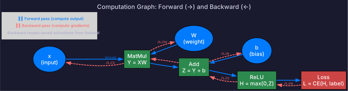
Gradients flow backward:

\frac{\partial L}{\partial \mathbf{x}} = \frac{\partial L}{\partial \mathbf{h}_2} \cdot \frac{\partial \mathbf{h}_2}{\partial \mathbf{h}_1} \cdot \frac{\partial \mathbf{h}_1}{\partial \mathbf{x}}

In practice, automatic differentiation computes vector-Jacobian products — never materializing the full Jacobian matrix.

Linear Layer Backward Pass

For $\mathbf{Y} = \mathbf{X}\mathbf{W}$ with incoming gradient $\frac{\partial L}{\partial \mathbf{Y}}$ :

\frac{\partial L}{\partial \mathbf{X}} = \frac{\partial L}{\partial \mathbf{Y}} \cdot \mathbf{W}^\top, \qquad \frac{\partial L}{\partial \mathbf{W}} = \mathbf{X}^\top \cdot \frac{\partial L}{\partial \mathbf{Y}}

Both backward operations are matrix multiplies — same GEMM kernels as the forward pass. Backward is approximately 2× the compute of forward (two GEMMs vs one), which is why the rule of thumb is: total training FLOPs ≈ 3× forward FLOPs.

Softmax + Cross-Entropy: The Clean Gradient

The combined gradient of softmax cross-entropy has a remarkably simple form:

\frac{\partial L}{\partial z_i} = \hat{y}_i - y_i

For the correct class: $\hat{y}_c - 1$ . For all others: $\hat{y}_i$ . Just “prediction minus target.”

This is why fused softmax-cross-entropy kernels are both numerically stable AND computationally efficient — the gradient doesn’t require recomputing the full Jacobian.

5. Gradient Problems and Solutions

Gradient Vanishing and Exploding

In a deep network, backward gradients are products of many Jacobians:

\frac{\partial L}{\partial \mathbf{h}_1} = \prod_{k=1}^{N} \mathbf{J}_k \cdot \frac{\partial L}{\partial \mathbf{h}_N}

If $\|\mathbf{J}_k\| < 1$ for most layers → gradients vanish (early layers stop learning). If $\|\mathbf{J}_k\| > 1$ for most layers → gradients explode (training diverges).

Residual Connections

\mathbf{h}_{l+1} = \mathbf{h}_l + f(\mathbf{h}_l)

The gradient becomes:

\frac{\partial \mathbf{h}_{l+1}}{\partial \mathbf{h}_l} = \mathbf{I} + \frac{\partial f}{\partial \mathbf{h}_l}

The identity matrix $\mathbf{I}$ ensures gradients have a direct path through the network — even if $\frac{\partial f}{\partial \mathbf{h}_l}$ is small, the gradient doesn’t vanish. This is why every Transformer block uses residual connections.

LayerNorm and RMSNorm

LayerNorm normalizes across the hidden dimension:

\text{LN}(\mathbf{x}) = \gamma \odot \frac{\mathbf{x} - \mu}{\sqrt{\sigma^2 + \epsilon}} + \beta

RMSNorm (used in LLaMA, Qwen) skips mean centering:

\text{RMSNorm}(\mathbf{x}) = \gamma \odot \frac{\mathbf{x}}{\sqrt{\frac{1}{H}\sum x_i^2 + \epsilon}}

Both stabilize gradient magnitudes across layers. RMSNorm is ~10-15% faster (fewer operations) with comparable quality.

Gradient Clipping

If $\|\nabla\| > \text{threshold}$ , scale it down:

\nabla \leftarrow \nabla \cdot \frac{\text{threshold}}{\|\nabla\|}

A last-resort safety net. Modern LLM training typically clips at gradient norm 1.0.

Adam Optimizer

Adam is the optimizer used in virtually all LLM training. It maintains two running averages per parameter:

First moment $m_t = \beta_1 m_{t-1} + (1 - \beta_1) g_t$ \ (momentum \ gradient direction)
Second moment $v_t = \beta_2 v_{t-1} + (1 - \beta_2) g_t^2$ \ (adaptive learning rate per parameter)

With bias correction and update:

\hat{m}_t = \frac{m_t}{1 - \beta_1^t}, \quad \hat{v}_t = \frac{v_t}{1 - \beta_2^t}, \quad \theta_t = \theta_{t-1} - \alpha \frac{\hat{m}_t}{\sqrt{\hat{v}_t} + \epsilon}

Why this matters for infrastructure: Adam stores $m$ and $v$ for every parameter \ both in FP32. For a model with $N$ parameters:

Parameters: $2N$ bytes (BF16)
Gradients: $4N$ bytes (FP32)
Adam $m$ : $4N$ bytes (FP32)
Adam $v$ : $4N$ bytes (FP32)
FP32 master weights: $4N$ bytes
Total: 18 bytes per parameter

Typical values: $\beta_1 = 0.9$ , $\beta_2 = 0.999$ , $\epsilon = 10^{-8}$ , $\alpha = 10^{-4}$ to $10^{-5}$ .

AdamW (Adam with decoupled weight decay) is the standard variant for LLM training \ it separates weight decay from the gradient update.

6. Numerical Precision and Mixed-Precision Training

Floating-Point Is a Finite Set

Every floating-point format trades off dynamic range (exponent bits) vs precision (mantissa bits). See GPU Evolution & Tensor Cores for the full format comparison and bit layout diagram.

The key tradeoff for training: BF16 has the same dynamic range as FP32 (8 exponent bits) but less precision (7 mantissa bits). FP16 has more precision (10 mantissa bits) but much smaller range (max 65,504 — easily overflows).

\text{fl}(w + \delta) = w

The update is silently dropped. This is why optimizers keep FP32 master weights — low-precision weights would swallow small gradient updates.

Non-Associativity

Due to rounding at each step:

\text{fl}(\text{fl}(a + b) + c) \neq \text{fl}(a + \text{fl}(b + c))

Parallel reductions using tree-structured addition may produce slightly different results with different thread counts or block sizes. This is not a bug — but results must be within acceptable error bounds.

Mixed-Precision Training Pattern

Mixed Precision Flow

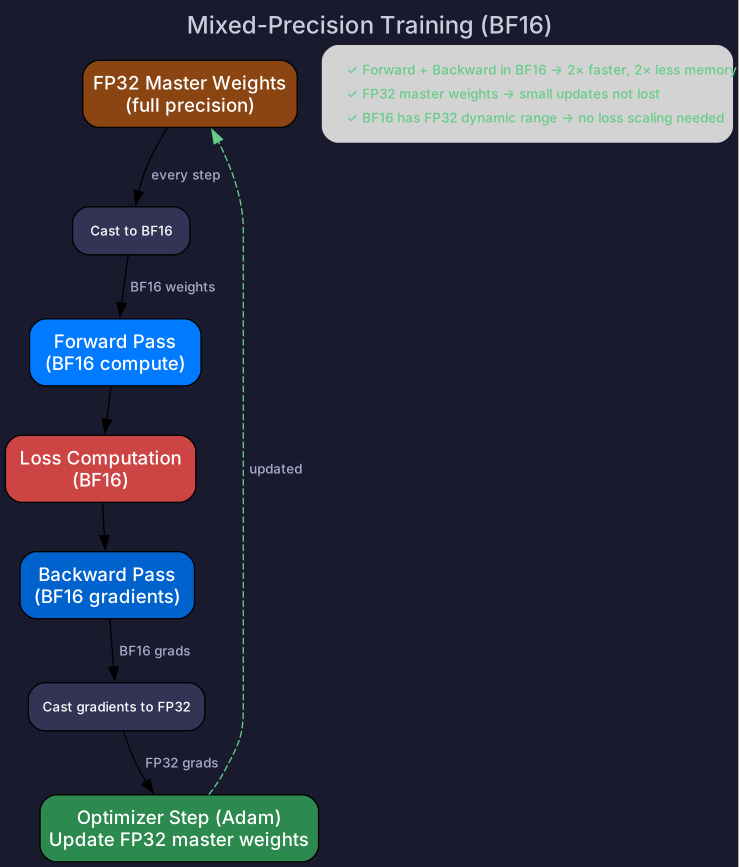
The standard recipe:

Forward: compute in BF16 (fast, fits in memory)
Backward: compute gradients in BF16
Update: accumulate in FP32 master weights (preserves small updates)

FP32 master weights → cast to BF16 → forward → backward (BF16 gradients)
         ↑                                              ↓
         └──────── FP32 optimizer update ←──── cast gradients to FP32

Why BF16 over FP16: BF16 has the same dynamic range as FP32, so it rarely overflows. FP16 maxes at 65,504 — a single large activation can overflow, requiring loss scaling (multiply loss by a large constant before backward, then divide gradients after). BF16 eliminates this complexity.

Loss Scaling (FP16 only)

When using FP16, small gradients underflow to zero. Loss scaling artificially inflates them:

Multiply loss by scale factor $S$ (e.g., 1024)
Backward pass computes scaled gradients: $S \cdot \nabla L$
Divide gradients by $S$ before the optimizer step
If overflow is detected, skip the update and halve $S$

Dynamic loss scaling adjusts $S$ automatically. But this is extra infrastructure complexity — another reason BF16 is now preferred.

Self-Check

Explain why raw logits need softmax before they’re probabilities
Implement numerically stable softmax (subtract max first)
Explain why fused log_softmax + cross_entropy is both faster and more stable
Write the backward pass for a linear layer $\mathbf{Y} = \mathbf{X}\mathbf{W}$
Explain why training FLOPs ≈ 3× forward FLOPs
Explain gradient vanishing and how residual connections solve it
Explain why BF16 is preferred over FP16 for training
Explain why FP32 master weights are needed with BF16 training
Explain non-associativity and why parallel reductions can produce different results