Self-Attention Mechanism

Self-attention is the computational heart of every LLM — the most FLOPs-intensive, most memory-hungry, and most optimized operation in the entire stack. Understanding it deeply is essential for everything from kernel engineering to serving optimization.

0. A Brief History of Attention

Before Self-Attention, sequence models relied on RNNs/LSTMs which processed tokens sequentially — creating a bottleneck for long sequences and preventing parallelization.

Bahdanau Attention (2014): Added attention to RNN encoder-decoder for translation. The decoder could “look back” at any encoder position instead of relying on a single fixed-length vector.
Luong Attention (2015): Simplified the attention score computation (dot product instead of learned alignment).
Self-Attention (2017, “Attention Is All You Need”): Removed RNNs entirely. Every token attends to every other token in parallel. This unlocked massive parallelism on GPUs and became the foundation of all modern LLMs.

The key insight: attention replaces sequential processing with parallel matrix operations — exactly what GPUs are built for.

1. The QKV Framework

Self-attention uses three projections of the same input to create a retrieval system:

Query (Q): “what am I looking for?”
Key (K): “what do I contain?” (used for matching)
Value (V): “what information do I provide?” (used for output)

Think of it like a library: Q is your search query, K is the index card on each book, V is the book’s content. You match your query against all index cards, then read the most relevant books.

Linear Projections

\mathbf{Q} = \mathbf{X}\mathbf{W}_Q, \quad \mathbf{K} = \mathbf{X}\mathbf{W}_K, \quad \mathbf{V} = \mathbf{X}\mathbf{W}_V

Each is a GEMM: $(B, S, d) \times (d, d) \to (B, S, d)$ .

Implementation optimization: In practice, $\mathbf{W}_Q$ , $\mathbf{W}_K$ , $\mathbf{W}_V$ are fused into a single matrix $\mathbf{W}_{QKV}$ of shape $(d, 3d)$ , computed as one GEMM then split — better GPU utilization.

2. Scaled Dot-Product Attention

Five steps, each with clear shape tracking:

Step 1: Compute Attention Scores

\mathbf{S} = \mathbf{Q}\mathbf{K}^\top \qquad (B, N_h, S, d_k) \times (B, N_h, d_k, S) = (B, N_h, S, S)

Element $S_{ij}$ is the dot product between token $i$ ‘s query and token $j$ ‘s key — how much token $i$ should attend to token $j$ .

This produces the $S \times S$ attention matrix — the source of attention’s $O(S^2)$ complexity.

Step 2: Scale

\mathbf{S} = \frac{\mathbf{S}}{\sqrt{d_k}}

Without scaling, dot products grow with dimension $d_k$ , pushing softmax into saturation (near-zero gradients). Dividing by $\sqrt{d_k}$ keeps values in a range where softmax produces useful gradients.

Step 3: Causal Mask (Decoder Only)

Causal Mask

\mathbf{S} = \mathbf{S} + \mathbf{M}

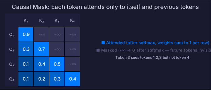
Where $\mathbf{M}$ is upper-triangular $-\infty$ :

M = [  0,  -∞,  -∞,  -∞ ]
    [  0,   0,  -∞,  -∞ ]
    [  0,   0,   0,  -∞ ]
    [  0,   0,   0,   0 ]

After softmax, $e^{-\infty} = 0$ — future tokens get zero attention weight. This enforces autoregressive generation: each token can only see itself and previous tokens.

Step 4: Softmax

\mathbf{A} = \text{softmax}(\mathbf{S}) \qquad \text{row-wise, each row sums to 1}

$A_{ij}$ is the attention weight from token $i$ to token $j$ .

Step 5: Weighted Sum

\text{Output} = \mathbf{A}\mathbf{V} \qquad (B, N_h, S, S) \times (B, N_h, S, d_k) = (B, N_h, S, d_k)

Each token’s output is a weighted combination of all (visible) value vectors, with weights determined by the attention scores.

Complete Formula

\text{Attention}(Q, K, V) = \text{softmax}\left(\frac{QK^\top}{\sqrt{d_k}} + M\right) V

3. Multi-Head Attention

Instead of one attention function with dimension $d$ , use $N_h$ heads each with dimension $d_k = d / N_h$ :

class MultiHeadSelfAttention(nn.Module):
    def __init__(self, d_model: int, num_heads: int):
        super().__init__()
        self.num_heads = num_heads
        self.head_dim = d_model // num_heads

        self.W_QKV = nn.Linear(d_model, 3 * d_model, bias=False)  # fused
        self.W_O = nn.Linear(d_model, d_model, bias=False)

    def forward(self, x, mask=None):
        B, S, d = x.shape

        # Fused QKV projection: one GEMM instead of three
        QKV = self.W_QKV(x)                          # (B, S, 3d)
        Q, K, V = QKV.chunk(3, dim=-1)               # each (B, S, d)

        # Reshape into heads: (B, S, d) → (B, Nh, S, dk)
        Q = Q.view(B, S, self.num_heads, self.head_dim).transpose(1, 2)
        K = K.view(B, S, self.num_heads, self.head_dim).transpose(1, 2)
        V = V.view(B, S, self.num_heads, self.head_dim).transpose(1, 2)

        # Attention scores: (B, Nh, S, dk) × (B, Nh, dk, S) → (B, Nh, S, S)
        scores = (Q @ K.transpose(-2, -1)) / (self.head_dim ** 0.5)
        if mask is not None:
            scores = scores.masked_fill(mask == 0, float('-inf'))
        attn = torch.softmax(scores, dim=-1)

        # Weighted sum: (B, Nh, S, S) × (B, Nh, S, dk) → (B, Nh, S, dk)
        out = attn @ V

        # Merge heads: (B, Nh, S, dk) → (B, S, d)
        out = out.transpose(1, 2).contiguous().view(B, S, d)

        return self.W_O(out)  # output projection

Why multiple heads? Each head learns a different attention pattern — one might track syntactic relationships, another semantic similarity, another positional proximity. The output projection $\mathbf{W}_O$ combines all heads.

4. Compute and Memory Cost

For a single attention layer with batch $B$ , sequence $S$ , $N_h$ heads, dimension $d_k$ :

Operation	FLOPs	Memory
QKV projections	$6BSd^2$	$3BSd$ (Q, K, V tensors)
$QK^\top$	$2BN_hS^2d_k$	$BN_hS^2$ (attention matrix)
Softmax	$O(BN_hS^2)$	In-place
Attention × V	$2BN_hS^2d_k$	$BSd$ (output)
Output projection	$2BSd^2$	$BSd$

Key bottleneck: the attention matrix is $BN_hS^2$ elements. For $B=1, N_h=32, S=128K$ :

Attention matrix: $32 \times 128K^2 \times 2$ bytes (FP16) = 1 TB — doesn’t fit in memory
This is why FlashAttention (which never materializes this matrix) is essential

FlashAttention: The Solution

The $BN_hS^2$ attention matrix is the reason FlashAttention exists. Instead of materializing the full matrix in HBM, FlashAttention:

Computes attention in tiles that fit in SRAM (shared memory)
Uses online softmax to accumulate results without the full matrix
Never writes the $S imes S$ matrix to HBM

Result: exact attention with $O(S)$ memory instead of $O(S^2)$ , and 2-4× faster due to reduced HBM access. Covered in depth in the CUDA > Attention Kernels module.

Self-Check

Explain the roles of Q, K, V and their intuition
Trace attention shapes step by step for given B, S, d, Nh values
Explain why scaling by $\sqrt{d_k}$ is necessary
Explain the causal mask and what happens to masked positions after softmax
Implement multi-head attention from scratch in PyTorch
Calculate attention memory for a given sequence length and explain why FlashAttention is needed