PyTorch Fundamentals

PyTorch is the dominant framework for AI training and the foundation for everything that follows — distributed training, inference engines, and custom kernels all build on PyTorch primitives. This chapter covers what an AI infrastructure engineer must understand: not just how to use PyTorch, but what’s happening under the hood.

---

1. Tensors

Creating Tensors

import torch

# From data
x = torch.tensor([1.0, 2.0, 3.0])

# Zeros/ones/random with shape
w = torch.randn(768, 3072)          # normal distribution
b = torch.zeros(3072)               # all zeros

# Like another tensor (same shape, dtype, device)
x_like = torch.zeros_like(w)

Shape Operations

x = torch.randn(2, 3, 768)

x.view(6, 768)           # reshape (must be contiguous)
x.reshape(6, 768)        # reshape (copies if needed)
x.permute(1, 0, 2)       # reorder dimensions → (3, 2, 768)
x.unsqueeze(0)           # add dimension → (1, 2, 3, 768)
x.squeeze()              # remove all size-1 dimensions

# Transpose: no data copy, just changes stride
x.transpose(0, 1)        # (3, 2, 768) — stride changes, data stays
x.transpose(0, 1).contiguous()  # now actually rearranges memory

view fails on non-contiguous tensors (e.g., after transpose). Use reshape which handles both cases — but be aware it may copy.

Device Management

# Move to GPU
x_gpu = x.to('cuda')
x_gpu = x.cuda()              # shorthand
x_gpu = x.to('cuda:1')        # specific GPU

# Move to CPU
x_cpu = x_gpu.cpu()

# Check device
print(x_gpu.device)           # cuda:0

# Create directly on GPU
w = torch.randn(768, 768, device='cuda')

Common bug: operating on tensors from different devices throws a runtime error. In distributed training, every tensor must be on the correct GPU.

dtype and Memory

x = torch.randn(1000, 1000)                           # FP32: 4 MB
x_fp16 = x.half()                                      # FP16: 2 MB
x_bf16 = x.to(torch.bfloat16)                         # BF16: 2 MB

# Memory per element
# FP32: 4 bytes | FP16/BF16: 2 bytes | FP8: 1 byte | INT8: 1 byte

---

2. Autograd: Automatic Differentiation

Computation Graph

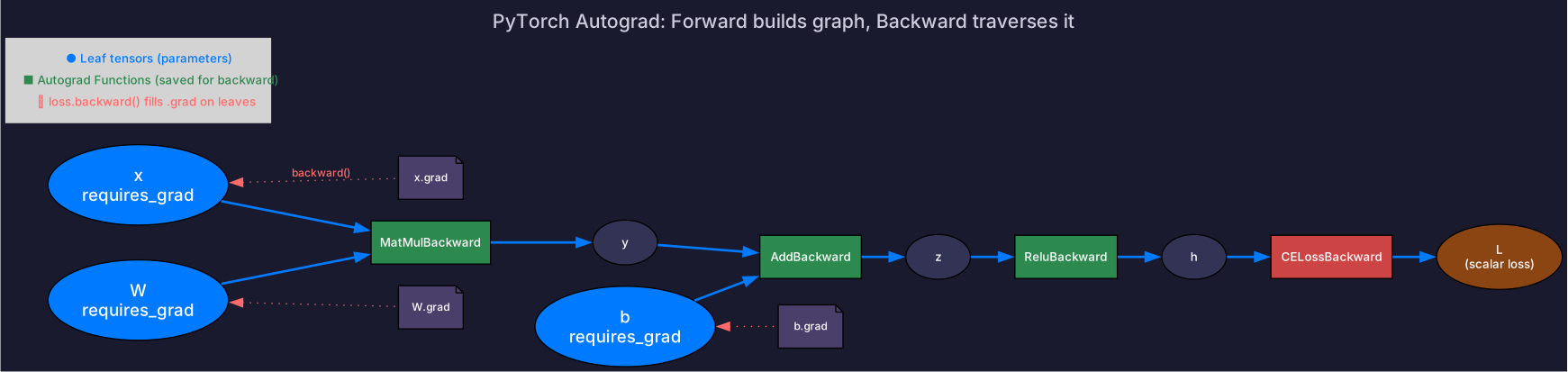
PyTorch builds a dynamic graph during the forward pass and uses it for backward:

x = torch.tensor(3.0, requires_grad=True)
y = x ** 2 + 2 * x + 1        # graph: x → square → add → add
y.backward()                    # traverse graph backward
print(x.grad)                  # 2*3 + 2 = 8.0

The graph is dynamic — rebuilt every forward pass. This is why PyTorch supports variable-length sequences and conditional logic naturally.

Gradient Accumulation and Zeroing

optimizer.zero_grad()          # MUST zero before backward
loss.backward()                # accumulates into .grad
optimizer.step()               # updates parameters

If you forget zero_grad(), gradients accumulate across iterations — a silent bug that produces wrong results.

Intentional accumulation is used for gradient accumulation (simulating larger batch sizes):

for i, batch in enumerate(dataloader):
    loss = model(batch) / accumulation_steps
    loss.backward()                        # gradients accumulate
    if (i + 1) % accumulation_steps == 0:
        optimizer.step()
        optimizer.zero_grad()

Disabling Gradient Tracking

# Inference: no gradients needed
with torch.no_grad():
    output = model(input)

# Evaluation mode: affects dropout, batchnorm
model.eval()

# Detach from graph (e.g., for target networks)
target = prediction.detach()

---

3. nn.Module: Model Organization

Defining a Model

import torch.nn as nn

class TransformerBlock(nn.Module):
    def __init__(self, hidden_size):
        super().__init__()
        self.norm1 = nn.LayerNorm(hidden_size)
        self.attn = nn.MultiheadAttention(hidden_size, num_heads=12)
        self.norm2 = nn.LayerNorm(hidden_size)
        self.ffn = nn.Sequential(
            nn.Linear(hidden_size, 4 * hidden_size),
            nn.GELU(),
            nn.Linear(4 * hidden_size, hidden_size),
        )

    def forward(self, x):
        x = x + self.attn(self.norm1(x), self.norm1(x), self.norm1(x))[0]
        x = x + self.ffn(self.norm2(x))
        return x

Parameter Inspection

# Count total parameters
total = sum(p.numel() for p in model.parameters())
trainable = sum(p.numel() for p in model.parameters() if p.requires_grad)
print(f"Total: {total:,} | Trainable: {trainable:,}")

# Save/load model
torch.save(model.state_dict(), "checkpoint.pt")
model.load_state_dict(torch.load("checkpoint.pt"))

---

4. The Training Loop

Standard Pattern

model = MyModel().cuda()
optimizer = torch.optim.AdamW(model.parameters(), lr=1e-4, weight_decay=0.01)
scheduler = torch.optim.lr_scheduler.CosineAnnealingLR(optimizer, T_max=1000)

for epoch in range(num_epochs):
    model.train()
    for batch in train_dataloader:
        input_ids = batch['input_ids'].cuda()
        labels = batch['labels'].cuda()

        # Forward
        logits = model(input_ids)
        loss = nn.functional.cross_entropy(logits.view(-1, vocab_size), labels.view(-1))

        # Backward
        optimizer.zero_grad()
        loss.backward()
        torch.nn.utils.clip_grad_norm_(model.parameters(), max_norm=1.0)
        optimizer.step()
        scheduler.step()

    # Evaluation
    model.eval()
    with torch.no_grad():
        # ... evaluate on validation set

DataLoader

from torch.utils.data import DataLoader, Dataset

dataloader = DataLoader(
    dataset,
    batch_size=32,
    shuffle=True,
    num_workers=4,          # parallel data loading (separate processes)
    pin_memory=True,        # faster CPU→GPU transfer
    prefetch_factor=2,      # prefetch 2 batches per worker
)

num_workers > 0 spawns separate processes (bypasses GIL). pin_memory=True uses page-locked memory for faster cuda() transfers. Both are essential for keeping GPUs fed.

Checkpointing

# Save
checkpoint = {
    'epoch': epoch,
    'model_state_dict': model.state_dict(),
    'optimizer_state_dict': optimizer.state_dict(),
    'loss': loss.item(),
}
torch.save(checkpoint, f'checkpoint_epoch{epoch}.pt')

# Resume
checkpoint = torch.load('checkpoint_epoch5.pt')
model.load_state_dict(checkpoint['model_state_dict'])
optimizer.load_state_dict(checkpoint['optimizer_state_dict'])
start_epoch = checkpoint['epoch'] + 1

---

5. GPU Memory and Mixed Precision

Monitoring GPU Memory

# In code
print(f"Allocated: {torch.cuda.memory_allocated() / 1e9:.2f} GB")
print(f"Reserved:  {torch.cuda.memory_reserved() / 1e9:.2f} GB")

# Detailed breakdown
print(torch.cuda.memory_summary())

# From command line
nvidia-smi
watch -n 1 nvidia-smi    # continuous monitoring

Allocated = memory actively used by tensors. Reserved = memory PyTorch grabbed from CUDA (includes cached blocks for reuse). If reserved >> allocated, PyTorch has fragmented memory.

Mixed Precision Training with AMP

from torch.amp import autocast, GradScaler

scaler = GradScaler()     # only needed for FP16, not BF16

for batch in dataloader:
    optimizer.zero_grad()

    # Forward in BF16
    with autocast(device_type='cuda', dtype=torch.bfloat16):
        logits = model(batch['input_ids'].cuda())
        loss = criterion(logits, batch['labels'].cuda())

    # Backward (scaler handles FP16 loss scaling; no-op for BF16)
    scaler.scale(loss).backward()
    scaler.step(optimizer)
    scaler.update()

Memory savings — a 7B model:

• FP32: ~28 GB for parameters alone
• BF16: ~14 GB for parameters
• With optimizer states, the difference is ~2×

---

6. Profiling

torch.profiler

from torch.profiler import profile, record_function, ProfilerActivity

with profile(
    activities=[ProfilerActivity.CPU, ProfilerActivity.CUDA],
    record_shapes=True,
    with_stack=True,
) as prof:
    with record_function("training_step"):
        logits = model(input_ids)
        loss = criterion(logits, labels)
        loss.backward()

# Print top operations by GPU time
print(prof.key_averages().table(sort_by="cuda_time_total", row_limit=10))

# Export for Chrome trace viewer
prof.export_chrome_trace("trace.json")

Common Performance Problems

Symptom	Likely Cause	Fix
Low GPU utilization (< 80%)	CPU data loading bottleneck	Increase num_workers, use pin_memory
GPU utilization spikes/drops	Small batch size, sync overhead	Increase batch size, use gradient accumulation
OOM on first batch	Model too large for GPU	Mixed precision, gradient checkpointing, ZeRO
OOM mid-training	Activation memory grows	Fixed sequence length, activation checkpointing
Slow first iteration	CUDA kernel compilation (JIT)	Warmup iteration, torch.compile cache

torch.cuda.synchronize() before timing — CUDA operations are asynchronous. Without sync, you’re measuring launch time, not execution time.

---

7. torch.compile: Graph-Mode Optimization

torch.compile (PyTorch 2.0+) captures the computation graph and optimizes it:

model = torch.compile(model)  # one line
output = model(input)          # first call: compile + run (slow)
output = model(input)          # subsequent: run optimized code (fast)

What it does under the hood:

1. TorchDynamo: captures Python bytecode into a graph
2. TorchInductor: compiles the graph into optimized Triton/C++ kernels
3. Operator fusion: merges multiple ops into fewer kernel launches

Typical speedup: 10-40% for training, more for inference. Limitations: dynamic shapes may cause recompilation; not all Python patterns are capturable.

---

8. Distributed Training Preview

A minimal preview of multi-GPU training (covered in depth in the Distributed module):

import torch.distributed as dist
from torch.nn.parallel import DistributedDataParallel as DDP

# Initialize process group (one process per GPU)
dist.init_process_group(backend='nccl')
local_rank = int(os.environ['LOCAL_RANK'])
torch.cuda.set_device(local_rank)

# Wrap model in DDP
model = MyModel().cuda(local_rank)
model = DDP(model, device_ids=[local_rank])

# Training loop is identical — DDP handles gradient sync
for batch in dataloader:
    loss = model(batch)
    loss.backward()       # DDP automatically AllReduces gradients
    optimizer.step()

Launch with: torchrun --nproc_per_node=8 train.py

DDP replicates the model on each GPU and synchronizes gradients after every backward pass via NCCL AllReduce.

---

Self-Check

• Create a tensor on GPU with specific dtype and shape
• Explain the difference between view and reshape
• Explain why optimizer.zero_grad() is necessary
• Implement gradient accumulation for N steps
• Count parameters in a model and estimate memory in FP32 vs BF16
• Set up DataLoader with num_workers and pin_memory
• Use torch.cuda.memory_summary() to diagnose memory usage
• Profile a training step and identify the top GPU operations
• Explain why torch.cuda.synchronize() is needed for accurate timing

---

References

• PyTorch Tutorials
• PyTorch Internals — Edward Z. Yang
• Automatic Mixed Precision — PyTorch Docs
• PyTorch Profiler — Tutorial