Scaling Laws

Scaling laws are the closest thing AI has to physics — they predict model quality from compute budget before you train. Understanding them is essential for capacity planning, hardware procurement, and deciding “should we train a bigger model or get more data?”

---

1. The Core Relationship

Model quality (measured by loss $L$) follows a power law in three variables:

$$L(N, D, C) \approx \left(\frac{N_c}{N}\right)^{\alpha_N} + \left(\frac{D_c}{D}\right)^{\alpha_D} + L_\infty$$

Where:

• $N$ = number of model parameters
• $D$ = number of training tokens
• $C$ = compute budget (FLOPs)
• $L_\infty$ = irreducible loss (entropy of the data)

More parameters, more data, and more compute all reduce loss — but with diminishing returns (power law, not linear).

---

---

2. Kaplan Scaling Laws (OpenAI, 2020)

The first systematic study of scaling. Key findings:

Power Law Relationships

$$L(N) \propto N^{-0.076}, \qquad L(D) \propto D^{-0.095}, \qquad L(C) \propto C^{-0.050}$$

Interpretation: Doubling parameters reduces loss by ~5%. Doubling data reduces loss by ~7%. Doubling compute reduces loss by ~3.5%.

Important: these predict loss (cross-entropy), not downstream task quality. A model with 5% lower loss may or may not be noticeably better at coding or reasoning. Loss is a necessary but not sufficient metric.

Kaplan’s Compute-Optimal Allocation

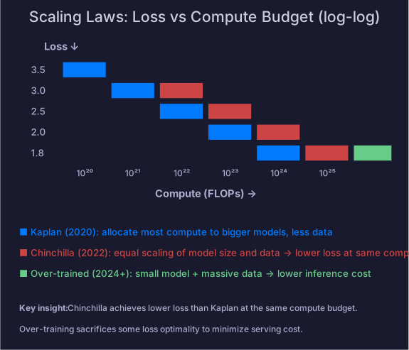
Given a fixed compute budget $C$, Kaplan suggested allocating most compute to larger models trained on relatively less data:

$$N_{\text{opt}} \propto C^{0.73}, \qquad D_{\text{opt}} \propto C^{0.27}$$

This means: when you get 10× more compute, make the model ~5.4× bigger but only train on ~1.9× more data.

This led to GPT-3 (175B parameters, 300B tokens) — very large model, relatively little data.

---

3. Chinchilla (DeepMind, 2022): The Correction

Chinchilla challenged Kaplan’s allocation by training over 400 models at different N/D ratios with the same compute budget, then fitting the optimal allocation curve. Key finding: Kaplan under-trained models.

Chinchilla’s Optimal Ratio

$$D_{\text{opt}} \approx 20 \times N$$

For a given compute budget, the optimal strategy is roughly equal scaling of parameters and data:

$$N_{\text{opt}} \propto C^{0.50}, \qquad D_{\text{opt}} \propto C^{0.50}$$

Model	Parameters	Training tokens	Tokens/param ratio	Status
GPT-3	175B	300B	1.7×	Under-trained (Kaplan)
Chinchilla	70B	1.4T	20×	Compute-optimal
LLaMA-1-65B	65B	1.4T	22×	~Chinchilla optimal
LLaMA-2-70B	70B	2.0T	29×	Over-trained
LLaMA-3-70B	70B	15T	214×	Massively over-trained

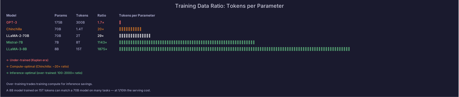
Chinchilla showed that GPT-3 should have been a 70B model trained on 5× more data, achieving the same quality at ~1/3 the inference cost (smaller model = cheaper to serve).

---

4. Beyond Compute-Optimal: Why Production Models Over-Train

If Chinchilla says 20 tokens per parameter is optimal, why does LLaMA-3 train at 214× tokens/param?

Because compute-optimal is NOT inference-optimal.

Chinchilla optimizes for: given a fixed training budget, minimize loss.

Production optimizes for: given a fixed inference cost, maximize quality.

The Inference Tax

A 70B model costs ~2× per request to serve compared to a 7B model. If you can train a 7B model to match 70B quality by using 10× more training data, the total cost drops:

Strategy	Training cost	Inference cost/request	Total cost (1B requests)
70B Chinchilla-optimal	$10M	$0.02	$10M +$20M = $30M
7B over-trained (100× data)	$1M	$0.01	$1M +$10M = $11M

Over-training small models is almost always cheaper in production because inference cost dominates training cost — a frontier model serves billions of requests but is trained once.

This is why every recent production model is massively over-trained:

• LLaMA-3-8B: 15T tokens (1875× ratio)
• Mistral-7B: 8T tokens (1143× ratio)
• Qwen-2.5-7B: 18T+ tokens

Training Compute Formula

Total training FLOPs (approximate):

$$C \approx 6ND$$

Where $N$ = parameters, $D$ = tokens. The 6× factor accounts for forward (2×) + backward (4×) per token.

Model	N	D	C (FLOPs)	GPU-hours (H100)
7B, 1T tokens	7B	1T	$4.2 \times 10^{22}$	~6,000
70B, 2T tokens	70B	2T	$8.4 \times 10^{23}$	~120,000
405B, 15T tokens	405B	15T	$3.6 \times 10^{25}$	~5,000,000

---

Scaling Law Limitations

Scaling laws are powerful but have known blind spots:

1. Loss ≠ quality: Scaling laws predict cross-entropy loss, not benchmark scores or user satisfaction. A model can have lower loss but worse performance on specific tasks.

2. Emergent capabilities: Some abilities (multi-step reasoning, few-shot learning, code generation) appear suddenly at certain scales rather than following smooth power laws. You can’t predict when they’ll emerge from loss curves alone.

3. Architecture-dependent: Scaling exponents differ between architectures (dense vs MoE, Transformer vs SSM). Chinchilla’s 20× ratio was measured on dense Transformers — MoE models may have different optimal ratios.

4. Data quality matters more than quantity: The laws assume uniform data quality. In practice, training on higher-quality data shifts the curve — you get the same loss with fewer tokens. This is why data curation is as important as scaling.

---

5. Scaling Law Implications for Infrastructure

Capacity Planning

Scaling laws let you predict performance before training:

1. Train small models (1B, 3B) at different token budgets
2. Fit the power law curve
3. Extrapolate to predict quality of the target model
4. Decide: bigger model or more data?

This saves millions of dollars — you don’t waste a 10K-GPU cluster on a bad configuration.

Hardware Procurement

The scaling equation $C \approx 6ND$ directly maps to hardware:

$$\text{Training time} = \frac{C}{\text{num\_GPUs} \times \text{FLOPS\_per\_GPU} \times \text{MFU}}$$

For a 70B model on 2T tokens with 1,000 H100s at 40% MFU:

$$\frac{8.4 \times 10^{23}}{1000 \times 989 \times 10^{12} \times 0.4} \approx 2.1 \times 10^6 \text{ seconds} \approx 24 \text{ days}$$

The Data Wall

As models over-train further, quality improvement per additional token diminishes. The field may be approaching a data wall — not enough high-quality text data exists to keep scaling at current rates. This drives:

• Synthetic data generation — using models to generate training data
• Multi-epoch training — repeating data (with diminishing returns after ~4 epochs)
• Multimodal data — images, audio, video as additional training signal
• Inference-time compute — spending more compute at inference instead of training (reasoning models)

---

Self-Check

• State the Chinchilla-optimal token-to-parameter ratio
• Explain why GPT-3 was “under-trained” by Chinchilla’s analysis
• Explain why production models over-train (inference cost dominates)
• Estimate training FLOPs for a given model size and token count using $C \approx 6ND$
• Calculate training time given FLOPs, GPU count, FLOPS/GPU, and MFU
• Explain the data wall and strategies to address it

---

References

• Scaling Laws for Neural Language Models (Kaplan et al., 2020)
• Training Compute-Optimal Large Language Models (Hoffmann et al., 2022 — Chinchilla)
• LLaMA: Open and Efficient Foundation Language Models (Touvron et al., 2023)
• Scaling Data-Constrained Language Models (Muennighoff et al., 2023)