The Transformer as a Compute Graph

Every optimization in AI infrastructure — kernel design, parallelism strategy, memory management — acts on some component of the Transformer. This chapter traces the complete forward pass of a decoder-only Transformer, tracking tensor shapes, data dependencies, and compute costs at every step. The goal: see the Transformer not as an abstract diagram but as a concrete sequence of matrix operations with measurable costs.

---

1. The Decoder-Only Architecture

Modern LLMs (GPT, LLaMA, Qwen, Mistral, DeepSeek) all use the decoder-only architecture. The full pipeline:

Input tokens → Embedding → N × Decoder Block → Final Norm → LM Head → Logits

End-to-End Data Flow

Tracing a single forward pass with concrete shapes:

Input: "What is attention" → Tokenizer → [1234, 567, 89]  (S=3 tokens)

Step 1: Token Embedding
  token_ids (B, S)  →  W_embed (V, d)  →  X (B, S, d)
  (1, 3)                (32000, 4096)      (1, 3, 4096)

Step 2: L × Decoder Block (shape preserved throughout)
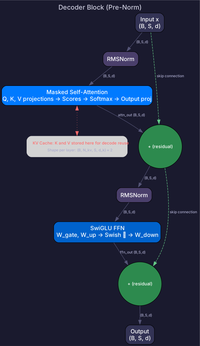
  ┌─ Block ──────────────────────────────────────────────┐
  │  x_norm = RMSNorm(X)                    (B, S, d)   │
  │  attn_out = MaskedSelfAttention(x_norm) (B, S, d)   │
  │  H = X + attn_out                ← residual         │
  │                                                      │
  │  h_norm = RMSNorm(H)                    (B, S, d)   │
  │  ffn_out = SwiGLU_FFN(h_norm)           (B, S, d)   │
  │  X_out = H + ffn_out             ← residual         │
  └──────────────────────────────────────────────────────┘
       × L layers (dimension stays (B, S, d) throughout)

Step 3: Final RMSNorm
  X_final (B, S, d)  →  RMSNorm  →  X_norm (B, S, d)

Step 4: LM Head
  X_norm (B, S, d)  ×  W_lm (d, V)  =  logits (B, S, V)
  (1, 3, 4096)         (4096, 32000)    (1, 3, 32000)

Step 5: Take last position, softmax → sample next token
  logits[:, -1, :]  →  softmax  →  sample  →  next token

Key observation: the hidden dimension $d$ is preserved through all L blocks. The only shape changes happen at input (token IDs → embeddings) and output (embeddings → vocabulary logits).

---

2. Inside a Decoder Block

Each decoder block has two sub-layers: masked self-attention and feed-forward network, each wrapped with normalization and residual connections.

Masked Self-Attention

$$\text{Attention}(Q, K, V) = \text{softmax}\left(\frac{QK^\top}{\sqrt{d_k}} + M\right)V$$

Where $M$ is the causal mask — an upper-triangular matrix of $-\infty$ that prevents attending to future tokens.

Step by step with shapes (for a single head):

Step	Operation	Shape
Input	$\mathbf{X}$	$(B, S, d)$
Q projection	$\mathbf{Q} = \mathbf{X}\mathbf{W}_Q$	$(B, S, d) \times (d, d) \to (B, S, d)$
K projection	$\mathbf{K} = \mathbf{X}\mathbf{W}_K$	$(B, S, d) \times (d, d) \to (B, S, d)$
V projection	$\mathbf{V} = \mathbf{X}\mathbf{W}_V$	$(B, S, d) \times (d, d) \to (B, S, d)$
Split heads	Reshape + transpose	$(B, N_h, S, d_k)$ where $d_k = d / N_h$
Attention scores	$\mathbf{Q}\mathbf{K}^\top / \sqrt{d_k}$	$(B, N_h, S, d_k) \times (B, N_h, d_k, S) \to (B, N_h, S, S)$
Causal mask	Add $-\infty$ to upper triangle	$(B, N_h, S, S)$
Softmax	Row-wise softmax	$(B, N_h, S, S)$
Weighted sum	$\text{Attn} \times \mathbf{V}$	$(B, N_h, S, S) \times (B, N_h, S, d_k) \to (B, N_h, S, d_k)$
Merge heads	Reshape	$(B, S, d)$
Output projection	$\mathbf{W}_O$	$(B, S, d) \times (d, d) \to (B, S, d)$

The $S \times S$ attention matrix is why attention is $O(S^2)$ in memory and compute — and why long-context serving is hard.

Feed-Forward Network (SwiGLU)

Modern LLMs use SwiGLU instead of the original ReLU FFN:

$$\text{FFN}(\mathbf{x}) = (\text{Swish}(\mathbf{x}\mathbf{W}_{\text{gate}}) \odot \mathbf{x}\mathbf{W}_{\text{up}}) \mathbf{W}_{\text{down}}$$

Step	Operation	Shape
Gate projection	$\mathbf{x}\mathbf{W}_{\text{gate}}$	$(B, S, d) \times (d, d_{ff}) \to (B, S, d_{ff})$
Up projection	$\mathbf{x}\mathbf{W}_{\text{up}}$	$(B, S, d) \times (d, d_{ff}) \to (B, S, d_{ff})$
Gate activation	$\text{Swish}(\text{gate}) \odot \text{up}$	$(B, S, d_{ff})$
Down projection	$\mathbf{W}_{\text{down}}$	$(B, S, d_{ff}) \times (d_{ff}, d) \to (B, S, d)$

SwiGLU has 3 weight matrices (gate, up, down) instead of 2 — this changes parameter counting.

RMSNorm

$$\text{RMSNorm}(\mathbf{x}) = \gamma \odot \frac{\mathbf{x}}{\sqrt{\frac{1}{d}\sum_{i=1}^{d} x_i^2 + \epsilon}}$$

Only $d$ learnable parameters (the scale $\gamma$). Compared to LayerNorm, RMSNorm skips mean centering — ~10-15% faster with comparable quality. Used by LLaMA, Qwen, Mistral, and most modern LLMs.

---

3. Model Configurations

Different model sizes use the same decoder block — just with different dimensions:

Model	$d$	$N_h$	$N_{kv}$	$d_k$	$L$	$d_{ff}$	$V$	Attention
LLaMA-2-7B	4096	32	32	128	32	11,008	32,000	MHA
LLaMA-2-13B	5120	40	40	128	40	13,824	32,000	MHA
LLaMA-2-70B	8192	64	8	128	80	28,672	32,000	GQA
Mistral-7B	4096	32	8	128	32	14,336	32,000	GQA
DeepSeek-V3	7168	128	—	—	61	18,432	129,280	MLA + MoE

Patterns to notice:

• $d_k = 128$ is universal: every model uses 128-dim attention heads. Scaling up means more heads, not bigger heads.
• SwiGLU changes $d_{ff}$: standard Transformer uses $d_{ff} = 4d$. SwiGLU has 3 matrices instead of 2, so $d_{ff} \approx (8/3)d$ to keep parameter count similar. LLaMA-2-7B: $(8/3) \times 4096 = 10,923 \to 11,008$ (rounded to 256 for GPU alignment).
• GQA reduces KV heads: LLaMA-2-70B uses 8 KV heads for 64 Q heads — each group of 8 Q heads shares 1 KV head. This cuts KV cache by 8× with minimal quality loss.

---

4. Parameter Counting

Estimating parameters is a fundamental AI infra skill — it directly tells you memory requirements.

Per-Block Parameters

For a single decoder block with MHA and SwiGLU:

Component	Formula	Count (7B, $d=4096$)
Q projection $\mathbf{W}_Q$	$d \times d$	16.8M
K projection $\mathbf{W}_K$	$d \times d$	16.8M
V projection $\mathbf{W}_V$	$d \times d$	16.8M
O projection $\mathbf{W}_O$	$d \times d$	16.8M
Gate $\mathbf{W}_{\text{gate}}$	$d \times d_{ff}$	45.1M
Up $\mathbf{W}_{\text{up}}$	$d \times d_{ff}$	45.1M
Down $\mathbf{W}_{\text{down}}$	$d_{ff} \times d$	45.1M
2× RMSNorm	$2d$	8.2K
Block total	$4d^2 + 3d \cdot d_{ff} + 2d$	202M

Total Model Parameters

Component	Formula	Count (LLaMA-2-7B)
Embedding	$V \times d$	131M
$L$ blocks	$L \times P_{\text{block}}$	32 × 202M = 6,464M
Final RMSNorm	$d$	4K
LM Head	$d \times V$	131M (often tied with embedding)
Total		~6.7B

With GQA (LLaMA-2-70B)

When $N_{kv} < N_h$, K and V projections shrink:

$$P_{\text{attn}} = d \cdot (N_h \cdot d_k) + 2 \cdot d \cdot (N_{kv} \cdot d_k) + (N_h \cdot d_k) \cdot d$$

For 70B: $N_h=64, N_{kv}=8, d_k=128, d=8192$:

• Q and O: $2 \times 8192 \times 8192 = 134M$
• K and V: $2 \times 8192 \times 1024 = 16.8M$
• Attention per block: 150.8M (vs 268M with full MHA — 44% reduction)

---

5. FLOP Counting

For a forward pass with batch size $B$, sequence length $S$, and model parameters:

Per-token compute (single decoder block):

Operation	FLOPs
QKV + O projections	$8BSd^2$
Attention scores $QK^\top$	$2BN_hS^2d_k$
Attention × V	$2BN_hS^2d_k$
FFN (SwiGLU, 3 matrices)	$6BSd \cdot d_{ff}$
Block total	$\approx 8BSd^2 + 4BS^2d + 6BSd \cdot d_{ff}$

For the full model with $L$ layers:

$$\text{Forward FLOPs} \approx L \times (8BSd^2 + 4BS^2d + 6BSd \cdot d_{ff})$$

Training FLOPs ≈ 3× forward (1× forward + 2× backward).

For LLaMA-2-7B ($d=4096, d_{ff}=11008, L=32, S=2048, B=1$):

• Per-token: ~14 GFLOPs
• Full sequence: ~28 TFLOPs
• The $S^2$ term (attention) is small at $S=2048$ but dominates at $S=128K$+

---

6. Why Decoder-Only Won

The original Transformer (2017) had both an encoder and decoder. Three architecture families emerged:

Architecture	Examples	Design	Status
Encoder-only	BERT, RoBERTa	Bidirectional attention, masked token prediction	Superseded for generation
Encoder-Decoder	T5, BART	Encoder processes input, decoder generates output	Used for translation, summarization
Decoder-only	GPT, LLaMA, Qwen	Causal attention, next-token prediction	Dominant for LLMs

Why decoder-only won:

1. Simpler: one architecture for both understanding and generation — no separate encoder
2. Scalable: just stack more identical blocks. No encoder-decoder cross-attention complexity
3. Unified pretraining: next-token prediction works for every task when prompted correctly
4. Efficient inference: KV cache works naturally with causal attention; encoder-decoder requires managing two caches

Every major production LLM today (GPT-4, Claude, LLaMA, Qwen, Mistral, DeepSeek) is decoder-only.

---

7. Depth vs Width: Scaling Dimensions

When scaling a model from 7B to 70B to 400B+, which dimensions change?

Dimension	7B (LLaMA-2)	70B (LLaMA-2)	405B (LLaMA-3.1)	Scaling pattern
$ (hidden)	4,096	8,192	16,384	~4×
$ (layers)	32	80	126	~4×
$ (heads)	32	64	128	~4×
$ (head dim)	128	128	128	Constant
{ff}$	11,008	28,672	53,248	Scales with $

Key patterns:

• Head dimension stays fixed at 128 — universally. More capacity = more heads, not bigger heads.
• Depth and width scale together — roughly doubling both gives ~8× parameters.
• Width affects per-layer cost quadratically (^2$ in attention projections) while depth affects cost linearly (more layers, same cost each).
• Depth gives more representational layers (more processing steps), width gives more capacity per layer (higher-dimensional representations).

In practice, scaling both gives the best quality per FLOP — this is what scaling laws predict.

---

Self-Check

• Trace the shape of a tensor through a complete forward pass (embedding → L blocks → logits)
• Explain why the hidden dimension $d$ is preserved through all blocks
• Explain the causal mask and why it prevents attending to future tokens
• Explain SwiGLU vs standard FFN (3 matrices vs 2, activation function)
• Calculate parameter count for a given model config
• Explain why $d_k = 128$ is universal and $d_{ff} \approx (8/3)d$ with SwiGLU
• Explain GQA and how it reduces KV cache
• Estimate forward FLOPs for a given model and sequence length

---

References

• Attention Is All You Need (Vaswani et al., 2017)
• LLaMA: Open and Efficient Foundation Language Models (Touvron et al., 2023)
• GLU Variants Improve Transformer (Shazeer, 2020)
• GQA: Training Generalized Multi-Query Transformer Models (Ainslie et al., 2023)