Multi-Model Serving

Not every query needs the largest model. Multi-model serving routes requests to the right model — saving cost while maintaining quality through intelligent routing and cascading.

---

1. Model Routing

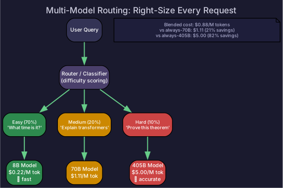
Difficulty-Based Routing

Classify query difficulty, route to appropriate model:

User query → Difficulty classifier (tiny model or heuristic)
  Easy (70%):  → 8B model (fast, cheap)
  Medium (20%): → 70B model (better quality)
  Hard (10%):  → 405B model (best quality)

Cost savings (compared to always using 70B):

$$\text{Routing cost} = 0.7 \times \$0.22 + 0.2 \times \$1.11 + 0.1 \times \$5.00 = \$0.88\text{/M tokens}$$

Compared to always using 70B ($1.11/M): **21$5.00/M): 82% savings. The actual savings depend on which model you would have used without routing.

Cascading

Try cheap model first, escalate if confidence is low:

Query → 8B model → confidence score
  If confidence > 0.9 → return 8B result (done)
  If confidence < 0.9 → 70B model → return 70B result

Advantage over routing: No separate classifier needed — use the model’s own confidence. Disadvantage: Latency for escalated queries (two model calls).

---

2. LoRA Multiplexing

Serve many fine-tuned variants on a shared base model:

Base model: Llama-3.1-70B (loaded once, shared)
  + LoRA adapter: customer_A (medical)
  + LoRA adapter: customer_B (legal)
  + LoRA adapter: customer_C (code)
  + ... hundreds of adapters

Each request: base_forward + adapter_forward (tiny extra cost)

Memory: 1 base model (140 GB) + 100 adapters (100 × 100 MB = 10 GB) = 150 GB total vs 100 × 140 GB = 14 TB if each customer got their own model.

For multi-adapter serving details, see Multi-Adapter Serving.

---

3. Model Co-Location

Run multiple models on the same GPU pool:

GPU 0-3: Llama-70B (TP=4) — handles complex queries
GPU 4:   Llama-8B — handles simple queries
GPU 5:   Embedding model — handles RAG retrieval
GPU 6:   Whisper — handles audio transcription
GPU 7:   Reranker — handles search reranking

Challenge: Memory allocation and scheduling between models. When the 70B model is idle, its GPU memory can’t easily be used by other models.

Dynamic Model Loading

Peak hours: Load 70B on 4 GPUs
Off-peak: Unload 70B, load 2× 8B instances (higher throughput for simple queries)

---

4. Cost-Quality Pareto Curve

For a given quality target, find the cheapest configuration:

Configuration	Quality (MMLU)	Cost/M tokens	Notes
405B BF16, TP=8	88%	$5.00	Maximum quality
70B INT4, TP=2	82%	$1.11	Good quality, 4.5× cheaper
8B INT4, 1 GPU	68%	$0.22	Simple tasks only, 23× cheaper
Cascading (8B → 70B)	80%	$0.55	Near-70B quality at half cost
Routing (8B/70B/405B)	85%	$0.80	Best cost/quality balance

The Pareto-optimal strategy depends on your quality threshold and budget.

---

Self-Check

• Design a difficulty-based routing strategy with 3 model sizes
• Calculate cost savings from cascading (70% simple, 30% complex queries)
• Explain LoRA multiplexing’s memory advantage over per-customer model copies
• Plot a cost-quality Pareto curve for a given set of models