Quantization Fundamentals

Quantization reduces numerical precision — fewer bits per number means less memory and faster computation. But the devil is in the details: how you map floating-point values to low-bit representations determines whether quality is preserved or destroyed.

1. What Gets Quantized

Three things in an inference engine can be quantized:

Target	When it exists	Primary benefit	Notation
Weights	Fixed after training	Smaller model, less weight loading (decode speedup)	W4, W8
Activations	Change with each input	Enable low-precision Tensor Core math (GEMM speedup)	A8, A16
KV Cache	Grows with context	More concurrent requests in same memory	KV8, KV4

W4A16: weights in 4-bit, activations in 16-bit. W8A8: both in 8-bit. The notation tells you what’s quantized and to what precision.

Weight-only quantization (W4A16) helps decode because decode is memory-bound — fewer bytes to load means faster generation. Weight+activation quantization (W8A8) also speeds up prefill because both operands of the GEMM are low-precision.

2. Scale and Zero-Point

The Quantization Formula

Map floating-point values to integer codes:

q = \text{clip}\left(\text{round}(x / s) + z, \; q_{\min}, \; q_{\max}\right)

\hat{x} = s \cdot (q - z)

Where:

$s > 0$ : scale — spacing between adjacent representable values
$z$ : zero-point — the integer code that represents floating-point 0
$q$ : the quantized integer code
$\hat{x}$ : the dequantized approximation (not equal to $x$ — information is lost)

Symmetric Quantization ( $z = 0$ )

Zero maps to zero. The representable range is symmetric around 0:

s = \frac{\max|x|}{q_{\max}}, \qquad q = \text{clip}(\text{round}(x/s), -q_{\max}, q_{\max})

For INT8 symmetric: $q_{\max} = 127$ , range $[-127, 127]$ .

Pros: Simpler computation (no zero-point offset), faster kernels. Cons: Wastes codes if values are not symmetric (e.g., all-positive activations after ReLU).

Asymmetric Quantization ( $z \neq 0$ )

Maps the actual data range $[\min(x), \max(x)]$ to the full integer range:

s = \frac{\max(x) - \min(x)}{q_{\max} - q_{\min}}, \qquad z = q_{\min} - \text{round}(\min(x)/s)

Pros: Uses all codes efficiently. Cons: Extra computation for the zero-point offset.

Worked Example

Data: $x = [0.2, 0.5, 8.0, -0.1]$ , INT8 symmetric:

s = \frac{8.0}{127} = 0.063, \qquad q = \text{round}([3.2, 7.9, 127, -1.6]) = [3, 8, 127, -2]

Dequantized: $\hat{x} = [0.189, 0.504, 8.001, -0.126]$ . The outlier 8.0 forces a large scale, causing the small values (0.2, -0.1) to have large relative errors.

3. Quantization Granularity

How many values share one set of scale/zero-point:

Granularity	Scale sharing	Metadata cost	Accuracy
Per-tensor	One scale for entire weight matrix	Minimal	Worst (one outlier affects all)
Per-channel	One scale per output channel	$C_{\text{out}}$ scales	Good (isolates channel variation)
Per-group	One scale per $G$ weights within a channel	$C_{\text{out}} \times \lceil C_{\text{in}}/G \rceil$ scales	Best (local range fitting)

Per-group with $G=128$ is the standard for INT4 weight quantization (GPTQ, AWQ). It balances accuracy (local scale) with metadata overhead (one FP16 scale per 128 INT4 weights = 16 bits / 128 = 0.125 bits overhead per weight).

For Activations

Activations change with every input, so scales must be computed at runtime:

Per-tensor: one scale computed from the max of the entire activation tensor
Per-token: one scale per token (row of the activation matrix) — better for outlier tokens
Per-channel: one scale per feature dimension — matches weight per-channel quantization

4. Calibration

For post-training quantization, scales are computed from a calibration dataset — a small set of representative inputs run through the model to observe value distributions:

# Pseudocode for calibration
calibration_data = load_calibration_set(num_samples=128)
for batch in calibration_data:
    activations = model.forward_with_hooks(batch)  # capture intermediate values
    for layer_name, values in activations.items():
        update_scale_statistics(layer_name, values)

# After calibration: compute final scales
scales = {name: compute_optimal_scale(stats) for name, stats in statistics.items()}

Calibration quality matters: if the calibration data doesn’t represent production inputs, the scales may be wrong — outlier values not seen during calibration will be clipped at inference time.

5. PTQ vs QAT

Approach	When	How	Quality	Cost
PTQ (Post-Training)	After training, no retraining	Calibrate scales, quantize weights	Good for ≥4-bit	Minutes to hours
QAT (Quantization-Aware Training)	During or after training	Simulate quantization in forward pass, train to compensate	Better for ≤4-bit	Full training cost

PTQ is standard for serving — GPTQ, AWQ, SmoothQuant are all PTQ methods. QAT is used when PTQ quality isn’t sufficient (very low bit widths, or quality-critical applications).

6. The Outlier Problem

Quantization Grid

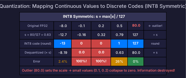
Transformer activations have outlier channels — a few feature dimensions with values 10-100× larger than others. These outliers make naive quantization fail:

Channel values: [0.1, 0.2, 0.3, 80.0, 0.1, 0.2]
                                   ↑ outlier!

INT8 symmetric scale: s = 80.0/127 = 0.63
Small values quantize to: 0.1/0.63 = 0.16 → rounds to 0
→ Most of the tensor is mapped to 0 or 1! Information destroyed.

Solutions (covered in following chapters):

SmoothQuant: Move outlier magnitude from activations to weights before quantizing
AWQ: Identify sensitive channels via activation statistics, protect them during weight quantization
Per-group quantization: Isolate outliers into their own group with a local scale
Mixed precision: Keep outlier channels in higher precision

For how SmoothQuant solves this for W8A8, see Weight-Activation Quantization. For weight-only approaches, see Weight-Only Quantization.

Self-Check

Write the quantization and dequantization formulas with scale and zero-point
Compare symmetric vs asymmetric quantization: when each is preferred
Calculate quantization error for a tensor with outliers
Explain per-tensor vs per-channel vs per-group granularity and their tradeoffs
Explain why calibration data matters and what happens with bad calibration
Compare PTQ vs QAT: cost, quality, and when to use each
Explain the outlier problem and name three solutions